
Data-Driven Astronomy
The following problems appeared as assignments in thecoursera courseData-Driven Astronomy.
One of the most widely used formats for astronomical images is theFlexible Image Transport System. In aFITSfile, the image is stored in a numerical array. TheFITS filesshown below are some of the publicly available ones downloaded from the following sites:
1. Computig the Mean and Median Stacks from a set of noisy FITS files
In this assignment, we shall focuss on calculating themeanof a stack of FITS files. Each individual file may or may not have a detected apulsar, but in the final stack we should be able to see aclear detection.
Computig the Mean FITS
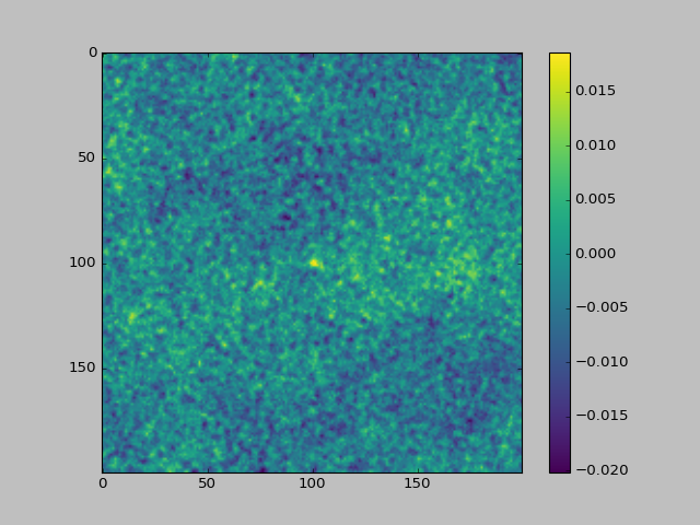
The following figure shows5 noisy FITSfiles, which will be used to compute themean FITSfile.

The following figure shows themean FITSfile computed from thes above FITS files. Mean being analgebraicmeasure, it€™s possible to computerunning meanby loadig each file at a time in the memory.
 Computing the Median FITS
Now let€™s look at a different statistical measure €” the median, which in many cases is considered to be a better measure than the mean due to its robustness to outliers. The median can be a more robust measure of the average trend of datasets than the mean, as the latter is easily skewed by outliers.
However, a naïve implementation of the median algorithm can bevery inefficientwhen dealing with large datasets.Median, being aholisticmeasure, required all the datasets to be loaded in memory for exact computation, when implemeted i a naive manner.
Calculating the median requires all the data to be in memory at once. This is an issue in typical astrophysics calculations, which may use hundreds of thousands of FITS files. Even with a machine with lots of RAM, it€™s not going to be possible to find the median of more than a few tens of thousands of images.This isn€™t an issue for calculating the mean, since the sum only requires one image to be added at a time.
Computing the approximate runing median: the BinApprox Algorithm
If there were a way to calculate a €œrunning median€ we could save space by only having one image loaded at a time. Unfortunately, there€™s no way to do an exact running median, but there are ways to do itapproximately.
Thebinapproxalgorithm does just this. The idea behind it is to find the median from the data€™s histogram.
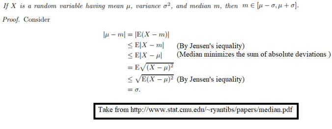
First of all it ca be proved that media always lies within one standard deviation of the mean, as show below:
The algorithm to find therunning approximate medianis show below:

As soon as the relevant bin is updated the data point being binned can be removed from memory. So if we€™re finding the median of a bunch ofFITSfiles we only need to have one loaded at any time. (The mean and standard deviation can both be calculated from running sums so that still applies to the first step).
The downside of usingbinapproxis that we only get an answer accurate toσ/Bby usingBbins. Scientific data comes with its own uncertainties though, so as long as you keep large enough this isn€™t necessarily a problem.
The following figure shows the histogram of1 milliondata points generated randomly. Now, thebinapproxalgorithm will be used to compute therunning medianand the error in approximation will be computed with different number of binsB.

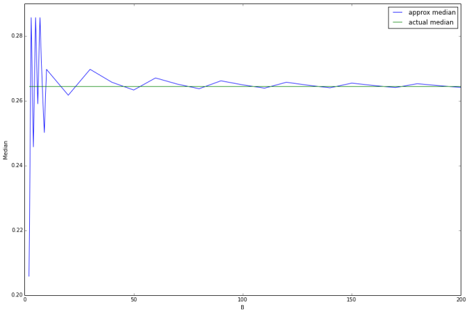

As can be seen from above, as the number of binsBincreases,theerrorin
approximationof the runningmediandecreases.
Now we can use thebinapproxalgorithm to efficiently estimate themedianof each pixel from a set of astronomy images inFITSfiles. The following figure shows10 noisy FITSfiles, which will be used to compute themedian FITSfile.

The following figure shows themedian FITSfile computed from the above FITS files using thebinapproxalgorithm.

2. Cross-matching
When investigating astronomical objects, likeactive galactic nuclei (AGN), astronomers compare data about those objects from different telescopes at different wavelengths.
This requires positionalcross-matchingto find the closest counterpart within a given radius on the sky.
In this activity you€™ll cross-match two catalogues: one from a radio survey, theAT20G Bright Source Sample (BSS) catalogueand one from an optical survey, theSuperCOSMOS all-sky galaxy catalogue.
The BSS catalogue lists the brightest sources from the AT20G radio survey while the SuperCOSMOS catalogue lists galaxies observed by visible light surveys. If we can find an optical match for our radio source, we are one step closer to working out what kind of object it is, e.g. a galaxy in the local Universe or a distant quasar.
We€™ve chosen one small catalogue (BSS has only 320 objects) and one large one (SuperCOSMOS has about 240 million) to demonstrate the issues you can encounter when implementing cross-matching algorithms.
The positions of stars, galaxies and other astronomical objects are usually recorded in either equatorial or Galactic coordinates.
Equatorial coordinates are fixed relative to the celestial sphere, so the positions are independent of when or where the observations took place. They are defined relative to the celestial equator (which is in the same plane as the Earth€™s equator) and the ecliptic (the path the sun traces throughout the year).
A point on the celestial sphere is given by two coordinates:
- Right ascension: the angle from the vernal equinox to the point, going east along the celestial equator;
- Declination: the angle from the celestial equator to the point, going north (negative values indicate going south).
The vernal equinox is the intersection of the celestial equator and the ecliptic where the ecliptic rises above the celestial equator going further east.
- Right ascension is often given in hours-minutes-seconds (HMS) notation, because it was convenient to calculate when a star would appear over the horizon. A full circle in HMS notation is 24 hours, which means 1 hour in HMS notation is equal to 15 degrees. Each hour is split into 60 minutes and each minute into 60 seconds.
- Declination, on the other hand, is traditionally recorded in degrees-minutes-seconds (DMS) notation. A full circle is 360 degrees, each degree has 60 arcminutes and each arcminute has 60 arcseconds.
Tocrossmatchtwo catalogs we need to compare the angular distance between objects on the celestial sphere.
People loosely call this a €œdistance€, but technically its an angular distance: the projected angle between objects as seen from Earth.
Angular distances have the same units as angles (degrees). There are other equations for calculating the angular distance but this one, called thehaversine formula, is good at avoiding floating point errors when the two points are close together.
If we have an object on the celestial sphere with right ascension and declination(α1,δ1), then the angular distance to another object with coordinates(α2,δ2)is given below:
 Before we cancrossmatchour two catalogs we first have to import the raw data. Every astronomy catalog tends to have its own unique format so we€™ll need to look at how to do this with each one individually.
We€™ll look at the AT20G bright source sample survey first. The raw data we€™ll be using is the file table2.dat from this page in the VizieR archives, but we€™ll use the filename bss.dat from now on.
Every catalogue in VizieR has a detailed README file that gives you the exact format of each table in the catalogue.
The full catalogue of bright radio sources contains 320 objects. The first few rows look like this:

The catalogue is organised in fixed-width columns, with the format of the columns being:
- 1: Object catalogue ID number (sometimes with an asterisk)
- 2-4: Right ascension in HMS notation
- 5-7: Declination in DMS notation
- 8-: Other information, including spectral intensities
The SuperCOSMOS all-sky catalogue is a catalogue of galaxies generated from several visible light surveys.
The original data is available on this pagein a package called SCOS_stepWedges_inWISE.csv.gz. The file is extracted to a csv file named super.csv.
The first few lines of super.csv look like this:

The catalog uses a comma-separated value (CSV) format. Aside from the first row, which contains column labels, the format is:
- 1: Right ascension in decimal degrees
- 2: Declination in decimal degrees
- 3: Other data, including magnitude and apparent shape.
Naive Cross-matcher
Let€™s implement a naivecrossmatchfunction that crossmatches two catalogs within a maximum distance and returns a list of matches and non-matches for the first catalog (BSS) against the second (SuperCOSMOS). The maximum distance is given in decimal degrees (e.g., nearest objects within a distance of5 degreewill be considered to be matched).
There are320objects in theBSScatalogthat are compared with firstnobjects from theSuperCOSMOScatalog. The values ofnis gradually increased from500to
1,25,000and impact on the running time and the number of matched objected are noted.
The below figures shows the time taken for thenaive cross-matchingas the umber of objects in thesecondcatalog is increased and also the final matches produced as abipartite graph.


An efficient Cross-Matcher
Cross-matching is a very common task in astrophysics, so it€™s natural that it€™s had optimized implementations written of it already. A popular implementation uses objects called k-d trees to perform crossmatching incredibly quickly, by constructing ak-d treeout of thesecond catalogue, letting it search through for a match for each object in thefirst catalogueefficiently. Constructing a k-d tree is similar to binary search: thek-dimensionalspace is divided into two parts recursively until each division only contains only a single object. Creating a k-d tree from an astronomy catalogue works like this:
- Find the object with the median right ascension, split the catalogue into objects left and right partitions of this
- Find the objects with the median declination in each partition, split the partitions into smaller partitions of objects down and up of these
- Find the objects with median right ascension in each of the partitions, split the partitions into smaller partitions of objects left and right of these
- Repeat 2-3 until each partition only has one object in it
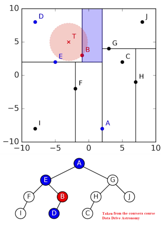
This creates a binary tree where each object used to split a partition (a node) links to the two objects that then split the partitions it has created (its children), similar to the one show in the image below.

Once ak-d treeis costructed out of a catalogue, finding a match to an object then works like this:
- Calculate the distance from the object to highest level node (the root node), then go to the child node closest (in right ascension) to the object
- Calculate the distance from the object to this child, then go to the child node closest (in declination) to the object
- Calculate the distance from the object to this child, then go to the child node closest (in right ascension) to the object
- Repeat 2-3 until you reach a child node with no further children (a leaf node)
- Find the shortest distance of all distances calculated, this corresponds to the closest object
Since each node branches into two children, a catalogue of objects will have, on average,log2(N)nodes from the root to any leaf, as show in the following figure.


As can be seen above, thekd-treebased implementation is way more faster than thenaivecounterpart for crossmatching. When thenaivetakes> 20 minsto match against1,25,000objects in thesecondcatalog, thekd-treebased implemetation takes just about1 secondto produce the same set of results, as shown above.