
We discuss a simple trick to significantly accelerate the convergence of an algorithm when the error term decreases in absolute value over successive iterations, with the error term oscillating (not necessarily periodically) between positive and negative values.
We first illustrate the technique on a well known and simple case: the computation of log 2 using its well know, slow-converging series. We then discuss a very interesting and more complex case, before finally focusing on a more challenging example in the context of probabilistic number theory and experimental math.
The technique must be tested for each specific case to assess the improvement in convergence speed. There is no general, theoretical rule to measure the gain, and if the error term does not oscillate in a balanced way between positive and negative values, this technique does not produce any gain. However, in the examples below, the gain was dramatic.
1. General framework and simple illustration
Let’s say you run an algorithm, for instance gradient descent. The input (model parameters) is x, the output if f(x), for instance a local optimum. We consider f(x) to be univariate, but it easily generalizes to the multivariate case, by applying the technique separately for each component. At iteration k, you obtain an approximation f(k, x) of f(x), and the error is E(k, x) = f(x) – f(k, x). The total number of iterations is N. starting with first iteration k = 1.
The idea consists in first running the algorithm as is, and then compute the “smoothed” approximations (moving averages), using the following m steps (with m em>N, typically, m = 3):
3.1. Convergence boosting scheme
- Step 1: Compute g(k, x, 1) = a f(k, x) + b f(k – 1, x) for k = 2, …, N
- Step 2: Compute g(k, x, 2) = a g(k, x, 1) + b g(k – 1, x, 1) for k = 3, …, N
- Step 3: Compute g(k, x, 3) = a g(k, x, 2) + b g(k – 1, x, 2) for k = 4, …, N
- …
- Step m: Compute g(k, x , m) = a g(k, x, m – 1) + b g(k – 1, x, m – 1) for k = m + 1, …, N
We must have a + b = 1. So far we only tested a = b = 1/2. We could also have a and b depend on the step and on the iteration k, but we haven’t tested yet adaptive a‘s and b‘s.
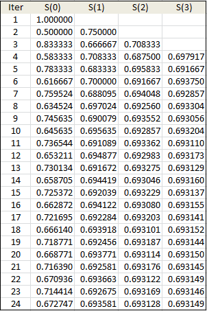
3.2. Example
See below the computation of f(x) = log x, with x = 2, m = 3, and N = 24. The result, up to 6 digits, is f(x) = 0.693147. Column S(0) in the table below is based on the raw formula log 2 = 1 – 1/2 + 1/3 – 1/4 + …, adding one term at each iteration k, that is,
Columns S(1), S(2), and S(3) correspond to the first 3 steps in the above scheme. While there are very efficient techniques to compute log 2 (see here), this simple trick allows you to gain more than one digit of accuracy per step. The standard algorithm yields one digit of accuracy when N = 24. Indeed, f(24, 2) = 0.672747. After just 3 steps, accuracy is up to 5 digits: g(24, 2, 3) = 0.693149.
3.3. Additional boosting
Note that we used a = b = 1/2 in our scheme, in the above example. If instead, we use a = 0.51 and b = 0.49, we obtain a substantial improvement: the last value in column S(1) becomes 0.693164, down from 0.693581. The true value is 0.693147 (approx.) It reduces the approximation error by a factor 25.
In order to find the optimum a (and b = 1 – a) for step 1, find a that minimizes | g(N, x, 1) – g(N – 1, x, 1) |. The same strategy can be used for step 2 as well, resulting in a = 0.30, b = 0.70 in this example (for step 2), again with a huge additional accuracy improvement.
2. A strange function
Unlike the logarithm for which very fast algorithms are available, the function below has no known miracle formula, and our trick may be the only option to boost convergence. Let
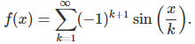
This function is rather peculiar. It is easy to establish the following:
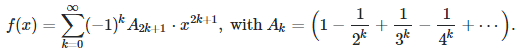
Note that A(1) = log 2, and for k > 1, we have
where ζ is the Riemann Zeta function. Also, f(−x) = −f(x) and we have the following approximation when x is large, using a value of K such that x / K < 0.01:
The function is smooth but exhibits infinitely many roots, maxima and minima, as well as slowly increasing oscillations as x increases. It is pictured below, with x between 0 and 200. More about it can be found here.

The computation for x = 316,547, yields f(x) = 18.81375 (approx.) Using the raw formula with the sine function, we get f(x) = 19.31352 after 205,443 iterations. Our trick provides the following gains:
- First step: f(x) = 18.81376 after 62,621 iterations
- Second step: f(x) = 18.81375 after 6,309 iterations
- Third step: f(x) = 18.81375 after 3,637 iterations
The charts below show improvement in convergence speed towards f(x) = 18.81375, using only N = 2,000 iterations, comparing the raw formula to compute f(316,547) at the top, versus 3 steps of our scheme at the bottom.
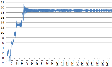
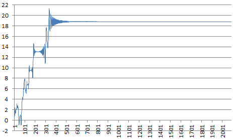
Interestingly, in all the cases tested with large values of x, the chaotic behavior in the above charts starts to stabilize and turns into smooth oscillations well before N reaches SQRT(x).
3. Even stranger functions
Here we are dealing with yet more peculiar functions that are nowhere continuous. Thus computing f(x) for various values around the target x and interpolating, would not help boost the speed of convergence or increase accuracy.
The first example is
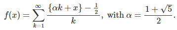
Here x is in [0, 1]. The brackets represent the fractional part function. This function is plotted below:
Try to approximate f(x) for various values of x, using our scheme to improve the slow speed of convergence. Is the series for f(x) always converging? The answer is yes, because of the equidistribution theorem and the fact that α is irrational.
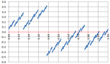
An even more challenging function is the following:
Again, x is in [0, 1]. This function is plotted below:
The choice of α and β is based on strong theoretical foundations, beyond the scope of this article. This function is related to the golden ratio numeration system. It converges for numbers that are normal in that system, and diverges for infinitely many numbers such as x = 3/5. However, normal numbers represent the vast majority of all numbers. If you pick up a number at random, the chance that it is normal is 100%. A number such as x = log 2 is conjectured to be normal in that system. Details can be found in Appendix B in my book Statistics: New Foundations, Toolkit, Machine Learning Recipes, available here, especially sections 3.2 and 4.3. In the golden ratio numeration system (a non-integer base system), digits are equal to 0 or 1, but the proportions of 0 and 1, unlike in the binary system, is not 50/50 for normal numbers.
Can you find a way to accelerate the convergence of this series? Note that due to machine precision, all terms beyond k = 60 will be erroneous if using standard arithmetic. One way to address this problem is to use high precision computing (Bignum libraries) as described in chapter 8 in my book Applied Stochastic Processes, available here.