
This is the continuation of my mini-series on sentiment analysis of movie reviews, which originally appeared on recurrentnull.wordpress.com. Last time, we had a look at how well classical bag-of-words models worked for classification of the Stanford collection of IMDB reviews. As it turned out, the “winner” was Logistic Regression, using both unigrams and bigrams for classification. The best classification accuracy obtained was .89 – not bad at all for sentiment analysis (but see the caveat regarding what’s good or bad in the first post).
Bag-of-words: limitations
So, bag-of-words models may be surprisingly successful, but they are limited in what they can do. First and foremost, with bag-of-words models, words are encoded using one-hot-encoding. One-hot-encoding means that each word is represented by a vector, of length the size of the vocabulary, where exactly one bit is “on” (1). Say we wanted to encode that famous quote by Hadley Wickham
Tidy datasets are all alike but every messy dataset is messy in its own way.
It would look like this:
| alike | all | but | dataset | every | in | is | its | messy | own | tidy | way | |
|---|---|---|---|---|---|---|---|---|---|---|---|---|
| 0 | 0 | 0 | 0 | 0 | 0 | 0 | 0 | 0 | 0 | 0 | 1 | 0 |
| 1 | 0 | 0 | 0 | 1 | 0 | 0 | 0 | 0 | 0 | 0 | 0 | 0 |
| 2 | 0 | 0 | 0 | 0 | 0 | 0 | 1 | 0 | 0 | 0 | 0 | 0 |
| 3 | 0 | 1 | 0 | 0 | 0 | 0 | 0 | 0 | 0 | 0 | 0 | 0 |
| 4 | 1 | 0 | 0 | 0 | 0 | 0 | 0 | 0 | 0 | 0 | 0 | 0 |
| 5 | 0 | 0 | 1 | 0 | 0 | 0 | 0 | 0 | 0 | 0 | 0 | 0 |
| 6 | 0 | 0 | 0 | 0 | 1 | 0 | 0 | 0 | 0 | 0 | 0 | 0 |
| 7 | 0 | 0 | 0 | 0 | 0 | 0 | 0 | 0 | 1 | 0 | 0 | 0 |
| 8 | 0 | 0 | 0 | 0 | 0 | 1 | 0 | 0 | 0 | 0 | 0 | 0 |
| 9 | 0 | 0 | 0 | 0 | 0 | 0 | 0 | 1 | 0 | 0 | 0 | 0 |
| 10 | 0 | 0 | 0 | 0 | 0 | 0 | 0 | 0 | 0 | 1 | 0 | 0 |
| 11 | 0 | 0 | 0 | 0 | 0 | 0 | 0 | 0 | 0 | 0 | 0 | 1 |
Now the thing is – with this representation, all words are basically equidistant from each other!
If we want to find similarities between words, we have to look at a corpus of texts, build a co-occurrence matrix and perform dimensionality reduction (using, e.g., singular value decomposition).
Let’s take a second example sentence, like this one Lev Tolstoj wrote after having read Hadley 😉
Happy families are all alike; every unhappy family is unhappy in its own way.
This is what the beginning of a co-occurrence matrix would look like for the two sentences:
| tidy | dataset | is | all | alike | but | every | messy | in | its | own | way | happy | family | unhappy | |
|---|---|---|---|---|---|---|---|---|---|---|---|---|---|---|---|
| tidy | 0 | 2 | 2 | 1 | 1 | 1 | 1 | 2 | 1 | 1 | 1 | 1 | 0 | 0 | 0 |
| dataset | 2 | 0 | 2 | 1 | 1 | 1 | 1 | 2 | 1 | 1 | 1 | 1 | 0 | 0 | 0 |
| is | 1 | 2 | 1 | 1 | 1 | 1 | 1 | 2 | 1 | 1 | 1 | 1 | 1 | 2 | 1 |
As you can imagine, in reality such a co-occurrence matrix will quickly become very, very big. And after dimensionality reduction, we will have lost a lot of information about individual words.
So the question is, is there anything else we can do?
As it turns out, there is. Words do not have to be represented as one-hot vectors. Using so-called distributed representations, a word can be represented as a vector of (say 100, 200, … whatever works best) real numbers.
And as we will see, with this representation, it is possible to model semantic relationships between words!
Before I proceed, an aside: In this post, my focus is on walking through a real example, and showing real data exploration. I’ll just pick two of the most famous recent models and work with them, but this doesn’t mean that there aren’t others (there are!), and also there’s a whole history of using distributed representations for NLP. For an overview, I’d recommend Sebastian Ruder’s series on the topic, starting with the first part on the history of word embeddings.
word2vec
The first model I’ll use is the famous word2vec developed by Mikolov et al. 2013 (see Efficient estimation of word representations in vector space).
word2vec arrives at word vectors by training a neural network to predict
- a word in the center from its surroundings (continuous bag of words, CBOW), or
- a word’s surroundings from the center word(!) (skip-gram model)
This is easiest to understand looking at figures from the Mikolov et al. article cited above:
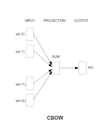
Fig.1: Continuous Bag of Words (from: Efficient estimation of word representations in vector space)
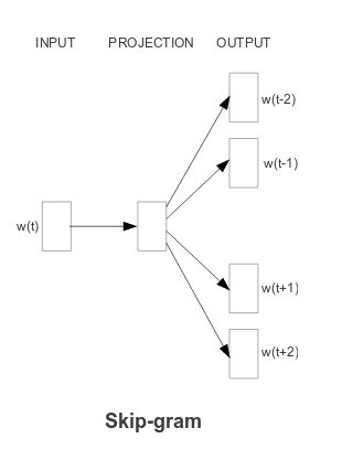
Fig.2: Skip-Gram (from: Efficient estimation of word representations in vector space)
Now, to see what is meant by “model semantic relationships”, have a look at the following figure:
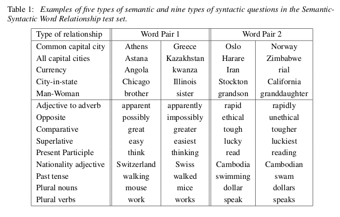
Fig. 3: Semantic-Syntactic Word Relationship test (from: Efficient estimation of word representations in vector space)
So basically what these models can do (with much higher-than-random accuracy) is answer questions like “Athens is to Greece what Oslo is to ???”. Or: “walking” is to “walked” what “swam” is to ???
Fascinating, right?
Let’s try this on our dataset.
Word embeddings for the IMDB dataset
In Python, word2vec is available through the gensim NLP library. There is a very nice tutorial how to use word2vec written by the gensim folks, so I’ll jump right in and present the results of using word2vec on the IMDB dataset.
I’ve trained a CBOW model, with a context size of 20, and a vector size of 100. Now let’s explore our model! Now that we have a notion of similarity for our words, let’s first ask: Which are the words most similar to awesome and awful, respectively? Start with awesome:
model.most_similar('awesome', topn=10) [(u'amazing', 0.7929322123527527), (u'incredible', 0.7127916812896729), (u'awful', 0.7072071433067322), (u'excellent', 0.6961393356323242), (u'fantastic', 0.6925109624862671), (u'alright', 0.6886886358261108), (u'cool', 0.679090142250061), (u'outstanding', 0.6213874816894531), (u'astounding', 0.613292932510376), (u'terrific', 0.6013768911361694)]
Interesting! This makes a lot of sense: So amazing is most similar, then we have words like excellent and outstanding.
But wait! What is awful doing there? I don’t really have a satisfying explanation. The most straightforward explanation would be that both occur in similar positions, and it is positions that the network learns. But then I’m still wondering why it is just awful appearing in this list, not any other positive word. Another important aspect might be emotional intensity. No doubt both words are very similar in intensity. (I’ve also checked co-occurrences, but those do not yield a simple explanation either.) Anyway, let’s keep an eye on it when further exploring the model. Of course we have to also keep in mind that for training a word2vec model, normally much bigger datasets are used.
These are the words most similar to awful:
model.most_similar('awful', topn=10) [(u'terrible', 0.8212785124778748), (u'horrible', 0.7955455183982849), (u'atrocious', 0.7824822664260864), (u'dreadful', 0.7722172737121582), (u'appalling', 0.7244443893432617), (u'horrendous', 0.7235419154167175), (u'abysmal', 0.720653235912323), (u'amazing', 0.708114743232727), (u'awesome', 0.7072070837020874), (u'bad', 0.6963905096054077)]
Again, this makes a lot of sense! And here we have the awesome – awful relationship again. On a close look, there’s also amazing appearing in the “awful list”.
For curiosity, I’ve tried to “subtract out” awful from the “awesome list”. This is what I ended up with:
model.most_similar(positive=['awesome'], negative=['awful']) [(u'jolly', 0.3947059214115143), (u'midget', 0.38988131284713745), (u'knight', 0.3789686858654022), (u'spooky', 0.36937469244003296), (u'nice', 0.3680706322193146), (u'looney', 0.3676275610923767), (u'ho', 0.3594890832901001), (u'gotham', 0.35877227783203125), (u'lookalike', 0.3579031229019165), (u'devilish', 0.35554438829421997)]
Funny … We seem to have entered some realm of fantasy story … But I’ll refrain from interpreting this result any further 😉
Now, I don’t want you to get the impression the model just did some crazy stuff and that’s all. Overall, the similar words I’ve checked make a lot of sense, and also the “what doesn’t match” is answered quite well, in the area we’re interested in (sentiment). Look at this:
model.doesnt_match("good bad awful terrible".split()) 'good' model.doesnt_match("awesome bad awful terrible".split()) 'awesome' model.doesnt_match("nice pleasant fine excellent".split()) 'excellent'
In the last case, I wanted the model to sort out the outlier on the intensity dimension (excellent), and that is what it did!
Exploring word vectors is fun, but we need to get back to our classification task. Now that we have word vectors, how do we use them for sentiment analysis?
We need one vector per review, not per word. What is done most often is to average vectors, and when we input these averaged vectors to our classification algorithms (the same as in the last post), this is the result we get (listing the bag-of-words results again, too, for easy comparison):
| Bag of words | word2vec | |
|---|---|---|
| Logistic Regression | 0.89 | 0.83 |
| Support Vector Machine | 0.84 | 0.70 |
| Random Forest | 0.84 | 0.80 |
So cool as our word2vec model is, it actually performs worse on classification than bag-of-words. Thinking about it, this is not so surprising, given that averaging over word vectors, we lose a whole lot of information – information we spent quite some calculation effort to obtain before… What if we already had vectors for a complete review, and didn’t have to average? Enter .. doc2vec – document (or paragraph) vectors! But this is already the topic for the next post … stay tuned!
:%20word2vec)