
I’ve had several folks tell me that if I can’t convert the “effects” in the Schmarzo “Economic Digital Asset Valuation Theorem” into mathematical equations, that my quest for a Nobel Prize in Economics would be greatly hindered. So, I enlisted the help of my senior data science team of Wei Lin, Mauro Damo and Yong Zhang to help me address this problem (they were only diverted from small projects related to preserving our rainforests, improving healthcare and reducing carbon emissions).
As a reminder, The Schmarzo “Economic Digital Asset Valuation Theorem” articulates why organizations need to invest in the creation, operationalization and reuse of their data and analytics digital assets. Data Silos and Orphaned Analytics are the great destroyers of the economic value of digital assets (see Figure 1).
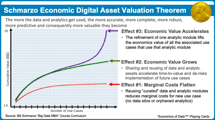
Figure 1: Schmarzo Economic Digital Value Asset Valuation Theorem
The Schmarzo “Economic Digital Asset Valuation Theorem” yields three economic “effects” that are unique for digital assets:
- Digital Asset Economic Effect #1: Marginal Costs Flatten. Since data never depletes, never wears out and can be reused at near zero marginal cost, the marginal costs associated with reusing data and analytic models flattens.
- Digital Asset Economic Effect #2: Economic Value Grows. Sharing and reusing of data and analytic models accelerate future use case time-to-value while de-risking implementation.
- Digital Asset Economic Effect #3: Economic Value Accelerates. Analytic model refinement (to improve analytic model accuracy, precision and recall) lifts the economic value of all associated use cases (that use that same analytic module).
Let’s look into the formulas that we created to support the Schmarzo Theorem…
Creating “Economic Digital Asset Valuation Theorem” Mathematical Equations
We went to work and found a website that converts mathematical equations into lines: https://www.mathe-fa.de/. Consequently, after much deliberation (and some manual chart manipulation), we came up with the following equations (see Figure 2):
- Effect #1: Marginal Costs Flatten: Red line: y = 1/(1+e^-x)-0.5
- Effect #2: Economic Value Grows: Green line: y = lg (x + 1)
- Effect #3: Economic Value Accelerates: Purple line: y = (x-2) ^ 3 + 8)
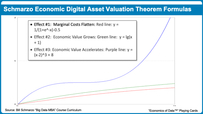
Figure 2: Mathematic Equations for Schmarzo Economic Digital Asset Valuation Theorem Effects
Nice. Very close to the lines Figure 1 (again, wish for some manipulation of the charting function).
Upon further inspection, it appears that Effect #3 is actually comprised of two components. The first component is the S curve driven by the re-use of improving Analytic Modules. The second effect is the compounding of small improvements in predictive accuracy, precision and recall of the Analytic Modules over a growing number of deployed use cases. Each use case that uses the improved Analytic Modules “inherits” any improvements in model accuracy, and those small improvements start to quickly compound into something significant (see Figure 3).
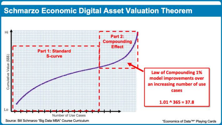
Figure 3: Two components of Effect #3
If folks have further suggestions to improve the mathematical formulas, I’d love to hear it. I’m going to have a long list of folks to thank when I collect that Nobel Prize!!