
Background
As part of my PhD work, I recently had to analyze any dataset(s) of my interest and present findings. I ended up conducting a study on US County-wise Covid-19 data. I wanted to share my key findings through this blog.
Study Question
The primary question I wanted to address through data analysis was “Do counties’ socioeconomic factors such as population size, poverty rate, unemployment rate, education percent and urbanization rate have any direct impact on the Covid-19 outbreak across counties within United States?”
Selected Datasets
- Covid-19 daily cases and deaths data for every county within United States (US) captured and published by the New York Times between January 1, 2020 and May 31 2020 (Coronavirus (Covid-19) data in the United States, 2020).
- Socioeconomic characteristics data such as population sizes, poverty, unemployment and education rates for every county within US captured and published by United States Department of Agriculture (USDA) (County-level socio-economic data in United States, 2020)
- Land area data for every county within US captured and published by United States Census Bureau (County-level land area data in United States, 2020)
- Urban-rural classification data for every county within US captured and published by United States Census Bureau (Counties’ urban-rural classification data in United States, 2020)
Data Details
- Covid-19 data: This data contained daily cases and deaths reported by each county across US captured between January 1, 2020 and May 31, 2020. Figure 1 below shows a snippet of the data.
- Counties’ population data: This data provided estimates of population for each US county captured between 2010 and 2019. Besides yearly estimates, this data contained many other estimates categorized by different demographics. For the purposes of current study, the 2019 estimate was used.
- Counties’ poverty data: This data provided estimates of poverty percentages for each US county which were last updated in 2018. There were several other estimates and metrics such as household incomes. For the purposes of current study, the overall poverty percentages updated in 2018 was used.
- Counties’ unemployment data: This data contained yearly unemployment rates for each US county captured between years 2000 and 2019. For the purposes of current study, the 2019 rates were used.
- Counties’ education data: This data provided percentages of population with less than high school diploma, with high school diploma, with some college degree and with bachelor’s degree or higher for every US county measured every decade starting in year 1970 and between years 2014 and 2018. For the purposes of this study, the percent with some college degree and the percent with bachelor’s or higher are used.
- Counties’ urban-rural data: This data provided population census based urban-rural classification data expressed in percentages for every US county. This data was captured for the decade in 2010 with incremental updates. The overall rural percent was considered.
- Counties’ land area data: This data provided land area in square miles for each US county captured every decade starting in 1990 and last updated in 2019. For the purposes of this study, 2019 values were used
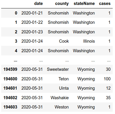 Figure 1: US Counties’ Covid-19 Cases By Date
Method
The method used in this analysis was to find correlations between US counties’ socioeconomic factors and the number of county-wise Covid-19 cases reported. The socioeconomic factors studied included population density, poverty rate, unemployment rate, education percent and urbanization percent. Correlation analysis is a statistical method that gives insights about existence of connections between quantitative variables and provides a metric to infer the strength of such relationships.
Analysis Tool
Jupyter Notebook was used to script the analysis steps using Python 3 programming language. While Python data analysis libraries such as NumPy, Pandas and Sklearn were used for data cleansing, integration, wrangling and executing correlations, Python’s plotting libraries such as Matplotlib and Seaborn were used to plot the results.
Analysis Steps
The steps involved extracting the required data fields from each dataset, cleansing the data, wrangling, additional fields computation and integration of data records to prepare data ready for executing correlational analysis. Cleansing of data involved imputation of missing values in different datasets and standardization of state and county fields so that records from different datasets can be mapped. Data wrangling involved collapsing and consolidating metric values and reshaping the datasets. Integration step involved matching records from all the processed datasets using state and county fields as unique keys to prepare consolidated dataset that is ready for analysis. Each dataset had county and state name fields. These two fields are used as primary keys to map records from different datasets. The final step involved executing the correlational analysis on the integrated dataset.
While poverty rate and unemployment rate were used directly from the respective datasets, the factors population density, education percent and urbanization percent were computed and derived. Population density was calculated as population size per square miles by using counties’ population estimates from population dataset and the counties’ land area from land area dataset. Education percent of a county was computed by adding percent with some college degree and percent with bachelor’s or higher degree found in the counties’ education rates dataset. Urban percent of a county was deduced by subtracting rural percent value from 100.
Data Preparation
The state and county fields in different datasets were represented in different formats. For example, the county field in different datasets had values such as ‘Baldwin County, Alabama’, ‘Baldwin County, AL’, ‘Baldwin, AL’ where state was either indicated as full name or using state code. In other datasets, the county field had values such as ‘Baldwin County’ and ‘Baldwin’ with state captured in separate field either using full name or state code.
As part of data preparation, county field was standardized to contain only the actual name part such as ‘Baldwin’. Similarly, the state field was standardized to contain only the state code such as ‘AL’. In case of datasets where state field had full name, the full name was transformed into a 2 letter state code.
Metric values in different datasets were on different scales. For example, total number of covid-19 cases was in hundreds of thousands, while population density values were in hundreds scale. It was challenging to visualize the data because data values with different scales could not fit the chart area. As such, there was a need to normalize and scale the data values specifically for visualization purposes. For example, logarithmic scale was used for total number of covid-19 cases, while min-max normalization coupled with a scaling factor used to visualize other metrics.
Results
Correlations were evaluated for all counties in US and separately for counties from top 4 states where the reported cases were higher. The top 4 states are New York, New Jersey, California and Illinois. Figure 2 below captures the correlations between the counties’ socioeconomic factors and total number of covid-19 cases.
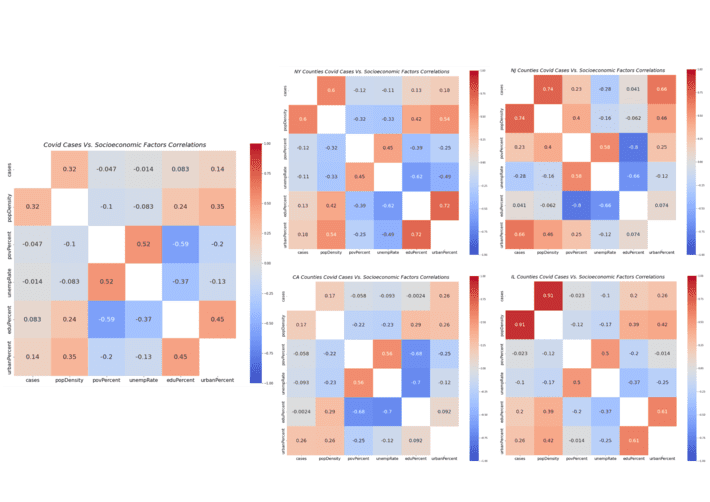 Figure 2: Correlation Matrices for All Counties, Counties in NY, NJ, CA, IL
Findings
- Population density manifested positive correlation with the total number of covid-19 cases. This was an expected result because it is generally believed that the outbreak was significant in highly populated counties
- State level correlations indicated that covid-19 impact was considerably higher in densely populated counties in New York, New Jersey and Illinois
- Socioeconomic factors such as poverty, unemployment and education rates did not manifest any correlations with the total number of covid-19 cases. However, there was observable positive correlation between poverty rates and covid-19 cases in New Jersey. The joint positive correlations of both population density and poverty rate in New Jersey, perhaps indicates that the impact of covid-19 was higher in highly populated counties with higher poverty rates
- Urban percentage manifested observable positive correlation with the total number of covid-19 cases. While urban percent showed strong positive correlation in New Jersey, it correlated significantly in the other three states. This result indicates that covid-19 impact was much higher in counties with lot more urbanization where typically higher population is expected
Other Findings
Results also showed correlations among the socioeconomic factors themselves. The following are key non-covid related inferences.
- Population density manifested higher degree of positive correlations with urban and education percents. From this it can be inferred that urban counties had populations with higher education levels
- Poverty rate manifested strong positive correlation with unemployment rates. This is perhaps an expected result since most counties with higher poverty rates also generally manifested higher unemployment rates
- Both poverty and unemployment rates manifested strong negative correlation with education percent. This indicates that most populations in counties with higher poverty and unemployment rates lacked college degree
Figure 3 below shows a scaled view of county-wise population density vs. covid-19 case in New York state.
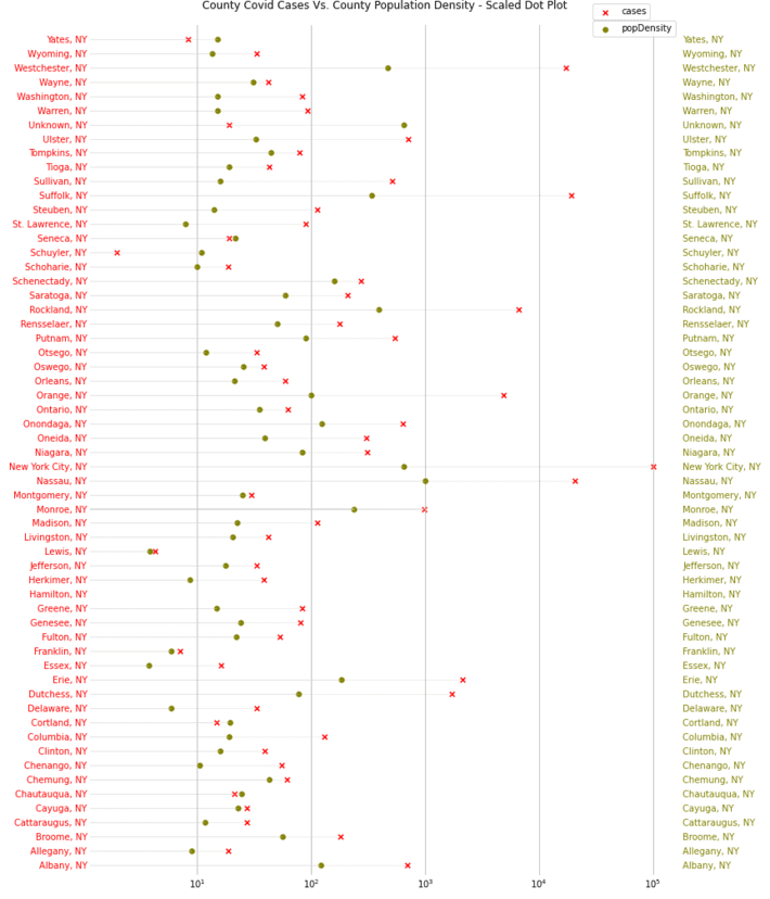 Figure 3: NY Counties’ Covid Cases Vs. Population Density Scaled Dot Plot
Key Inference
- Such insights can be used by decision makers in both healthcare and government organizations to plan, prepare and implement measures against such outbreaks. Such insights would also help decision makers identify vulnerable counties, particularly with higher populations and with higher urban areas, where there is higher possibility of outbreak as indicated by the results
- The findings also uncovered the need for more structured approaches to collect and process data for epidemiological outbreaks, need for a robust mechanism to collect such data in an automated fashion and a need for tools to conduct analysis and to assess actionable responses
Analysis Artifacts
If anyone is interested in the analysis artifacts, please message me on LinkedIn.
References
Coronavirus (Covid-19) data in the United States [Data set]. (2020). The New York Times. Retrieved from https://github.com/nytimes/covid-19-data
Counties’ urban-rural classification data in United States [Data set]. (2020). United States Census Bureau. Retrieved from https://www.census.gov/programs-surveys/geography/guidance/geo-area…
County-level land area data in United States [Data set]. (2020). United States Census Bureau. Retrieved from https://www.census.gov/library/publications/2011/compendia/usa-coun…
County-level socio-economic data in United States [Data set]. (2020). United States Department of Agriculture Economic Research Service. Retrieved from https://www.ers.usda.gov/data-products/county-level-data-sets/
Garattini, C., Raffle, J., Aisyah, D. N., Sartain, F., & Kozlakidis, Z. (2019). Big data analytics, infectious diseases and associated ethical impacts. Philosophy & Technology, 1, 69. http://dx.doi.org/10.1007/s13347-017-0278-y
Morgan, O. (2019). How decision makers can use quantitative approaches to guide outbreak responses. Philosophical Transactions of the Royal Society B: Biological Sciences, 374(1776), 1
Redding, D. W., Atkinson, P. M., Cunningham, A. A., Lo Iacono, G., Moses, L. M., Wood, J. L. N., & Jones, K. E. (2019). Impacts of environmental and socio-economic factors on emergence and epidemic potential of Ebola in Africa. Nature Communications, 10(1), 4531. http://dx.doi.org/10.1038/s41467-019-12499-6