
 As is known and seen from the series of blog posts, Apache Spark is a powerful tool with many useful libraries (like MLlib and GraphX) which deals with big data. Sometimes you have to work with data that has lots of relationships, and usual SQL databases are not the best option then. However, that’s when NoSQL databases come to action. They are more flexible, and will better represent data with numerous connections.
In the previous blog post, we have considered the Apache Spark GraphX tool but to illustrate its possibilities we have used a small graph object. In the real world, the graphs can be much bigger and more complicated. Therefore in this post, we will create a bigger graph, will store it in Neo4j database and will analyze it using Apache Spark GraphX tool, namely Pagerank algorithm.
To do this, we are going to load some data from csv files which contain words with corresponding parts of speech (nodes) and edges between them (edges have “with” property which means that words can be often seen in one sentence). At first, let’s prepare data using pandas. Then we will push this data to Neo4j database. And finally, we’ll integrate Neo4j with GraphX to load graph from Neo4j database and analyze it using Spark GraphX.
Preparing data using pandas
Before we start, make sure that you have previously installed pandas library. If you haven’t, type in console:
pip install pandas
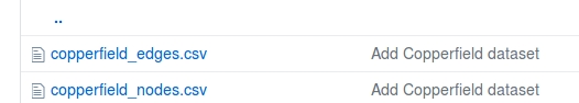
Also, you should download the dataset from here (you will need only the two files shown below):
It is necessary to say, that first of all we will read and clean up data in the python shell. So to launch python shell type in the console:
python
Before we read the data, let’s import pandas library:
import pandas as pd
Now, read csv files into respective DataFrames:
edges = pd.read_csv("copperfield_edges.csv")nodes = pd.read_csv("copperfield_nodes.csv")
To see the obtained DataFrames (for example, first 5 lines) – type the next command in python shell:
edges.head(5)
The output will be the following:
from to
0 man old
1 man person
2 old person
3 man anything
4 person anything
In the case of nodes:
nodes.head(5)
name part_of_speech
0 agreeable adjective
1 man noun
2 old adjective
3 person noun
4 anything noun
As we have said above, the copperfield_nodes.csv file contains words and their corresponding parts of speech, and the copperfield_edges.csv file contains connections between them.
Now we need to modify our data a little. The purpose is to mark all words in edges DataFrame with their parts of speech.
First of all, we need to merge our tables on words which the edges begin with:
from_tab = pd.merge( nodes, edges, left_on='name', right_on='from' )[['part_of_speech','from','to']]
The next step is to merge tables on words which the edge goes to:
to_tab = pd.merge(nodes, edges, left_on='name', right_on='to')[['part_of_speech','to','from']]
Let’s rename columns to exclude duplication (“pos” means part of speech):
from_tab.rename(columns = {"part_of_speech": "pos_from"}, inplace = True) to_tab.rename(
 columns = {"part_of_speech": "pos_to" }, inplace = True)
Finally, let’s merge tables to form the edges:
tab = pd.merge(from_tab, to_tab, on=["to","from"])[["pos_from","from","pos_to","to"]]
To see the first 5 lines of the obtained final table – type in the python shell:
tab.head(5)
The result should look like the following:
pos_from from pos_to to
0 noun man adjective old
1 noun man noun person
2 noun man noun anything
3 adjective old noun person
4 adjective old adjective bad
In this paragraph, we have prepared data, and now we can push it to the Neo4j graph database.
Loading data to Neo4j
First of all, you should install Neo4j. Neo4j can be downloaded from the official site. Community version will be enough for our purposes. When you click “DOWNLOAD” button you will be asked to submit a little form and after submitting you will be able to download Neo4j and will get the installation instruction which you should follow (the beginning of the instruction is shown on the screen below).
Note that the instruction is available only after downloading.

At the 2.2 step of the instruction, you will have to set the password. Here we’ll use a simple password: “password”. When you execute all steps of the instruction you will be able to install py2neo to connect to our Neo4j database from python.
Install py2neo:
pip install py2neo
At this step, you can connect to the database from python. But first, let’s make an import. In the python shell type:
from py2neo import Graph, Node, Relationship
Now we should create an empty graph in Neo4j database (“password” is the password that we have set earlier):
graph = Graph("bolt://localhost:7687",\auth=("neo4j", "password"))
And after that with the code below we can create our nodes and edges (relationships) and merge them into our previously created empty graph in Neo4j database:
for row in tab.iterrows():
node_a = Node(row[1][“pos_from”], name=row[1][“from”])
node_b = Node(row[1][“pos_to”], name=row[1][“to”])
rel = Relationship(node_a, “with”, node_b)
graph.merge(rel, “with”, “name”)
In case you want to drop the contents of your Neo4j database, use the following command:
graph.delete_all()
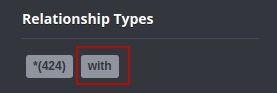
You can look at the visual graph representation using web interface by clicking “with” button, the colors of the nodes may differ from the presented below (you can change them manually):
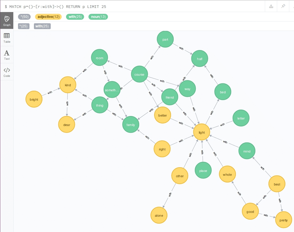
There is only a part of the whole graph in this figure because the whole graph is rather big and can not be shown in the web interface window. The colored circles with arrows mean the words with its connections to other words which can be used together in the sentences. As you can see yellow circles mean adjectives, green ones mean nouns.
Data analysis with Spark
We have saved the graph to Neo4j database, and now we can load it to Spark and perform its analysis using the PageRank algorithm to obtain the importance of each node. But firstly we should integrate Spark GraphX with Neo4j. Unfortunately, there is no python connector for GraphX yet, so we’ll have to deal with Scala. You’ll need the neo4j-spark connector.
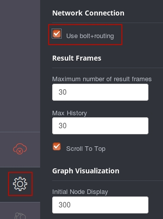
This connector uses a bolt interface, so you’ll have to turn it on. Go to http://localhost:7474, open settings (gear icon in the bottom-left corner) and switch “Use bolt+routing” to ON.
Now we can start spark-shell. We’ll have to specify our password for authentication, and include connector package:
./bin/spark-shell --conf spark.neo4j.bolt.password=password --packages neo4j-contrib:neo4j-spark-connector:2.2.1-M5
Next step is to make some imports for the further analysis:
import org.neo4j.spark._import org.apache.spark.graphx._import org.apache.spark.graphx.lib._
To connect to the Neo4j database, we need to create Neo4j instance:
val neo = Neo4j(sc)
To load graph from the Neo4j database, we should use Cypher, which is Neo4j’s query language. Using the query below, we will obtain the whole graph with all nodes and all edges:
val graphQuery = """MATCH (n)-[r]->(m)RETURN id(n) as source,id(m) as target, type(r) as value
 SKIP {_skip} LIMIT {_limit}"""
Now we can load the graph:
val graph: Graph[Long, String] = neo.rels(graphQuery).partitions(10).batch(200).loadGraph
It should be noted that the partitions and batch are optional parameters that can be used to define the level of parallelism.
Now we have loaded a graph, and it can be analyzed with Apache Spark GraphX tool. First of all, let’s perform the simplest operations. To count the vertices number in the graph type in the spark-shell:
graph.vertices.count
As a result, you will see the next line:
res0: Long = 111
To count the number of corresponding edges type:
graph.edges.count
The output will be the following:
res1: Long = 424
We can check these values by looking to the corresponding source files (“copperfield_nodes.csv”, “copperfield_edges.csv”).
As you can see such integration allows us to perform quick data processing over graphs using Spark GraphX tool. We can load data, process it and save back to the database. For example, let’s calculate the importance of each node using the PageRank algorithm and write these data back to the Neo4j database.
val g = PageRank.run(graph, 5)Neo4jGraph.saveGraph(sc, g, "rank")
In the first line “5” means the number of iterations.
To see the result using web interface ( press “rank” button to do this).
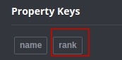
You should edit your Cypher query in the following way (take a look at the image below) and press Play:
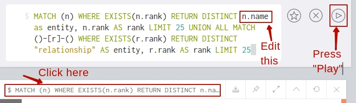
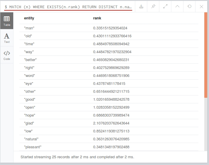
The result should look like the following:
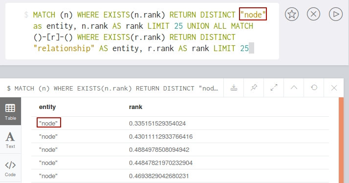
If you don’t do this, your query and results will look like:
Conclusions
Integration of Apache Spark GraphX tool with Neo4j database management system could be useful when you work with a huge amount of data with a lot of connections. Neo4j store the information in the graph format which reduces greatly the time which is needed for requests to the database. To explore the advantages of such an approach, we have built a trainee graph and pushed it to the Neo4j database. Then we have loaded this graph to Spark for the further analysis with the help of GraphX tool.
As a result, you can see that storing data in a graph format using Neo4j database has some benefits, including fast loading and easy visualization through the web interface.