
Guest blog post by Dalila Benachenhou, originally posted here. Dalila is Professor at George Washington University. In this article, benchmarks were computed on a specific data set, for Geico Calls Prediction, comparing Random Forests, Neural Networks, SVM, FDA, K Nearest Neighbors, C5.0 (Decision Trees), Logistic Regression, and Cart.
Introduction:
In the first blog, we decided on the predictors. In the second blog we pre-processed the numerical variables. We knew that different predictive models have different assumptions about their predictors. Random Forest has none, but Logistic Regression requires normality of the continuous variables, and assumes the probability between 2 consecutive unit levels in a series of numbers to stay constant. K Nearest Neighbors requires the predictors to be at least on the same scale. SVM, Logistic Regression, and Neural Networks tend to be sensitive to outliers. hence, we had to cater to these different predictive model assumptions and needs. We changed Predictors that need to be changed to categorical variables, or we made sure to scale them. We transformed Age and Tenure (the only 2 continuous variables) distributions to a normal distribution and then scaled and centered them. We came up with these 2 sets of predictors:
New_Predictors <- c=”” c_logins=”” p=”” ustomersegment=”” z_age=”” z_channel23m=”” z_channel33m=”” z_channel43m=”” z_channel53m=”” z_payments3m=”” z_tenure=””>
LR_new_predictors <- c=”” c_channel23m=”” c_channel33m=”” c_channel43m=”” c_channel53m=”” c_logins=”” c_payments3m=”” nbsp=”” p=”” ustomersegment=”” z_age=”” z_tenure=””>
LR_new_predictors are predictors for Logistic Regression. We used LR_new_predictors for both Logistic Regression, Random Forest, and K Nearest Neighbors.
Variables starting with z are at least scaled to 0 and 1 if they were discrete variables, or normalized scaled and centered, if they were continuous. Variables starting with c are the categorical form of the original variables. We decided on their number of levels by the significance of their odd ratios.
Method:
We decided to combine day15 and day16. From this combination, we split our dataset into Training set (80%), and Validation set (1/3 of 20%) , and Testing Set (2/3 of 20%). Due to the extreme class imbalance, we decided to use F1 Score to measure the models performance, and try 4 approaches to model building.
In the first approach, we used down sampling during model building, and found the maximum threshold with the validation set. We set the threshold to be the point where Sensitivity (Predict) and Positive Predictive Value (Recall) are highest in the ROC curve.
In the second approach, we down sampled during training phase, and tuned the models with a utility function during the validation phase. In the third approach, we built a C5.0 model with cost, and a Random Forest with a prior class probability and a utility function. In the fourth, and last, approach, we combined the models to create an “ensemble”.
For predictive models, in addition to Random Forest, and C5.0, we built a Neural Network, a Support Vector Machine with Radial Function, a K Nearest Neighbors, a Logistic Regression, a Flexible Discriminant Analysis (FDA) and a CART model.
PARAMETERS VALUES FOR THE PREDICTIVE MODELS:
Random Forest: mtry = 2, number of trees = 500
Neural Network: tried with : size = 1 to 10, decay values 0, 0.1, 1, and 2, and bag = FALSE
SVM : used RADIAL basis function Kernel with C (cost) = 1
FDA : degree = 1 and nprune= 1 to 25, the best nprune = 18
K Nearest Neighbors: k = 1 to 25, the best k = 20
C5.0 : Cost Matrix
|
No
|
Yes
|
|
|
No
|
5
|
-25
|
|
Yes
|
0
|
10
|
Logistic Regression : None
CART : default values
Results:
Many of you will be wondering why we have Random Forest. In the previous blog, we provided raw predictors to the Random Forest. In here, we provide the LR_new_predictors to the Random Forest. We want to see if pre-processed predictors result in a higher Random Forest performance. Except for Age and Tenure, the new_predictors are mostly categorical variables.
|
Yes Precision
|
No Precision
|
Yes Recall
|
No Recall
|
Yes F1 Score
|
No F1 Score
|
|
|
Random Forest
|
80.2
|
83.42
|
16.44
|
99.04
|
27.29
|
90.56
|
|
Neural Network
|
74.85
|
81.13
|
13.89
|
98.76
|
23.43
|
89.08
|
|
SVM
|
74.85
|
78.3
|
12.3
|
98.71
|
21.13
|
87.33
|
|
FDA
|
72.46
|
78.86
|
12.24
|
98.51
|
20.94
|
87.60
|
|
KNN
|
69.05
|
78.58
|
11.65
|
98.15
|
19.94
|
87.28
|
|
Logistic Reg
|
75.54
|
75.5
|
11.13
|
98.7
|
19.40
|
85.56
|
|
CART
|
73.65
|
74.96
|
10.69
|
98.59
|
18.67
|
85.17
|
|
Median
|
74.85
|
78.58
|
12.24
|
98.7
|
20.94
|
87.33
|
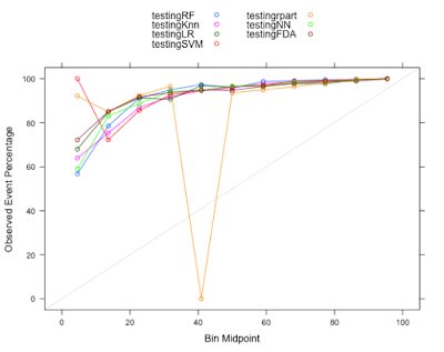
From the Calibration plot, except for CART (rpart package used), all the other models had good calibration and good performance.
In addition to this, we also used utility functions to improve Random Forest, Neural Network, SVM, and K Nearest Neighbors. In here we utilized down sampling, and then found a utility function using validation data set to tune our models.
|
Yes Precision
|
No Precision
|
Yes Recall
|
No Recall
|
Yes F1 Score
|
No F1 Score
|
|
|
Random Forest
|
72.46
|
90.77
|
24.2
|
98.78
|
36.28
|
94.6
|
|
Neural Network
|
70.66
|
80.03
|
12.58
|
98.53
|
21.36
|
88.32
|
|
KNN
|
67.07
|
78.96
|
11.48
|
98.33
|
19.6
|
87.59
|
|
SVM
|
77.84
|
73.65
|
10.73
|
98.79
|
18.86
|
84.39
|
Max Kuhn, Kjell Johnson, and many machine learning expert, we were told that the best approach is to down sample when building a predictive model. Still, we decided to build C5.0 with cost, and Random Forest with prior class probability and a utility function at the testing level. We were blown out by the result from Random Forest. The performance was extremely good, and better than all the other models. Yes, its Yes precision, and its No Recall values were lower than C5.0, but the F1 Score were much higher (79.88 vs 30.49) and (99.17 vs 91.70.)
|
Yes Precision
|
No Precision
|
Yes Recall
|
No Recall
|
Yes F1 Score
|
No F1 Score
|
|
|
Random Forest
|
80.83
|
99.12
|
78.94
|
98.21
|
79.88
|
99.17
|
|
C5.0
|
83.23
|
85.24
|
18.66
|
99.21
|
30.49
|
91.70
|
The utility function for the Random Forest is as follows:
|
No
|
Yes
|
|
|
No
|
5
|
-25
|
|
Yes
|
0
|
10
|
|
No
|
Yes
|
|
|
No
|
0
|
72
|
|
Yes
|
5
|
0
|
While the precision for Yes decreased, the Yes recall improved a lot. Now, for every Yes prediction, we have 24.2 that are true Yes. For SVM, we improved the Precision for Yes at the expense of the precision of No, and the Recall for Yes. For KNN we improved the Precision for
No, and slightly the F1 Score for No.
What if we use the majority wins approach to decide on our prediction:
|
Yes Precision
|
No Precision
|
Yes Recall
|
No Recall
|
Yes F1 Score
|
No F1 Score
|
|
|
Majority Wins
|
76.65
|
77.86
|
12.34
|
98.80
|
21.26
|
87.09
|
We will improve the Yes F1 Score, but we have a slight insignificant decrease in No F1 Score. For Yes Precision, the majority vote performance is lower only to Random Forest. For Yes Recall, the majority vote performance is lower than Random Forest and Neural Network Yes Recall. However, for No, the performance is higher only to Cart and Logistic Regression. In here, we have the get better prediction of the rarest event at the expense of the most common. A more sophisticated ensemble of all these predictive model will more likely produce better prediction that average.
Code:
results <- data.frame=”” rf=”newValuerf,” svm=”newValueSVM,</font”>
LR = newValueLR,rpart =newValuerpart,
KNN = newValueKnn,NN=newValueNN,FDA=newValueFDA)
for (i in 1:4273) {
m <- count=”” font=”” i=”” results=”” t=””>
l <- dim=”” font=”” m=””>
if (l[1] == 2) {
if ( m[1,2] > m[2,2]) {
outcome[i] = m[1,1]
}
else {
outcome[i] = m[2,1]
}
}
else {
outcome[i] = m[1,1]
}
}