
In 1927, W. O. Kermack y A. G. McKendrick described the first mathematical model for infectious diseases using a set of differential equations. This model is called SIR because of the three states one individual can have.
These states are:
- Susceptible: The individuals that can be infected by the disease
- Infected: The individuals that have been infected and suffer the disease.
- Recovered: The individuals that recovered from the disease and have become immune.
The equations that represent these states are as follows:
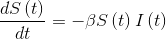
- Variation with time of the susceptible individuals to be infected will depend inversely on a transmission factor β and the susceptible population.

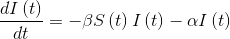
- Variation of those infected will depend on the number of people who are still susceptible of being infected, minus the number of people who have already recovered and are therefore immune.
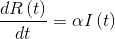
- The variation of recovered ones depends directly on the number of infected multiplied by α, a factor that determines the time that infected need to recover, that is:
The boundary conditions are:
- Population must always remain constantAt t=0
 At t=0

The analytical solution of this system can be found in different articles, for example here: arXiv:1403.2160
Instead of that, I will focus in equation (2) to note that it is a Bernoulli equation of the form

Where

The solution for this Bernoulli differential equation is the logistic function, which most general form is this:
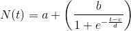
In the epidemiologic context, this logistic function represents the accumulative number of infected people as a function of time.
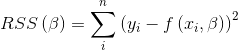
Using this model, it’s possible to fit it to the real data, to obtain the values for the variables, the way to do it consists in minimizing the residuals in the loss function
 Because the function to be fitted is not linear, the method to minimize de loss function must be suitable for nonlinear regressions. To do this regression, I used the NLS package for R, which implements the Gauss-Newton algorithm.
The data corresponds to the number of infected people in Spain as a function of time provided by the Ministry of Health.
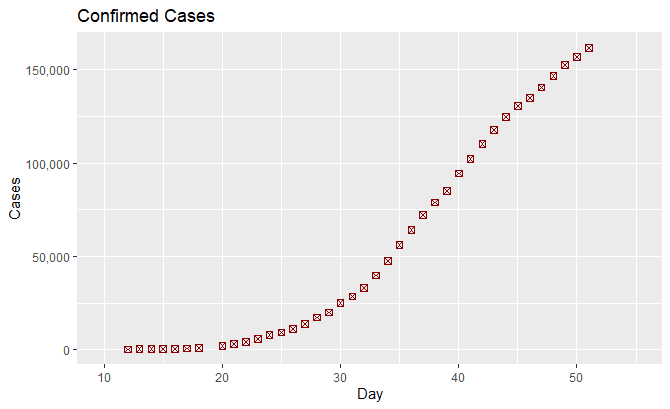 This graph represents the data.
How to execute the regression using R.
- Load the CSV with data using read_csv
descarga <- read_csv(“serie_historica_acumulados.csv”,col_types = colsFallecidos = col_double(), Fecha = col_date(format = “%d/%m/%Y”), Hospitalizados = col_double(), Recuperados = col_double(), UCI = col_double(), X8 = col_skip()))
- Group the data by date and sum all regions
agregados_por_fecha<-descarga %>% group_by(Fecha) %>% summarize(Fallecidos=sum(Fallecidos), Casos=sum(Casos), Hospitalizados=sum(Hospitalizados),UCI=sum(UCI), Recuperados=sum(Recuperados))
- Create a sequence to use it as a time scale
s<-seq(1:length(tabla_absolutos$Fecha))
tabla_absolutos[“dia”] <- s
- Use nls to fit the curve. To have a good fit, it is necessary to provide initial data compatible with the data. This need to be made manually.
logis.m1 <- nls(Casos ~ logis(dia, a, b, c,d), data = agregados_por_fecha, start = list(a = 0, b = 180000, c = 40, d=5))
- Use summary to retrieve the details of the regression.
summary(logis.m1)
Formula: Casos ~ logis(dia, a, b, c, d)
Parameters:
Estimate Std. Error t value Pr(>|t|)
a -2.320e+03 5.344e+02 -4.342 0.000115 ***
b 1.788e+05 2.111e+03 84.706 < 2e-16 ***
c 3.914e+01 1.317e-01 297.217 < 2e-16 ***
d 5.362e+00 1.033e-01 51.920 < 2e-16 ***
—
Signif. codes: 0 ‘***’ 0.001 ‘**’ 0.01 ‘*’ 0.05 ‘.’ 0.1 ‘ ’ 1
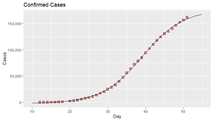 This graph represents the data and the regression curve.
Conclusions:
- The regression found the values for the variable that are compatible withe the data.
- The inflexion point occurred on day 39 (march29)
- The maximum number of infected people will be 180.000 people
- The number of infected will grow until May 15th.