

In this blog, we shall discuss about how to build a neural network to translate from English to German. This problem appeared as the Capstone project for the coursera course Tensorflow 2: Customising your model, a part of the specialization Tensorflow2 for Deep Learning, by the Imperial College, London. The problem statement / description / steps are taken from the course itself. We shall use the concepts from the course, including building more flexible model architectures, freezing layers, data processing pipeline and sequence modelling.

Image taken from the Capstone project
Here we shall use a language dataset from http://www.manythings.org/anki/ to build a neural translation model. This dataset consists of over 200k pairs of sentences in English and German. In order to make the training quicker, we will restrict to our dataset to 20k pairs. The below figure shows a few sentence pairs taken from the file.

Our goal is to develop a neural translation model from English to German, making use of a pre-trained English word embedding module.
1. Text preprocessing
We need to start with preprocessing the above input file. Here are the steps that we need to follow:
- First lets create separate lists of English and German sentences.
- Add a special and token to the beginning and end of every German sentence.
- Use the Tokenizer class from the tf.keras.preprocessing.text module to tokenize the German sentences, ensuring that no character filters are applied.
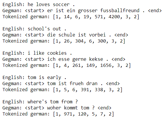
The next figure shows 5 randomly chosen examples of (preprocessed) English and German sentence pairs. For the German sentence, the text (with start and end tokens) as well as the tokenized sequence are shown.
- Pad the end of the tokenized German sequences with zeros, and batch the complete set of sequences into a single numpy array, using the following code snippet.
padded_tokenized_german_sentences = tf.keras.preprocessing.sequence.pad_sequences(tokenized_german_sentences, maxlen=14, padding='post', value=0) padded_tokenized_german_sentences.shape #(20000, 14)
As can be seen from the next code block, the maximum length of a German sentence is 14, whereas there are 5743 unique words in the German sentences from the subset of the corpus. The index of the <start> token is 1.
max([len(tokenized_german_sentences[i]) for i in range(20000)]) # 14 len(tokenizer.index_word) # 5743 tokenizer.word_index[''] # 1
2. Preparing the data with tf.data.Dataset
Loading the embedding layer
As part of the dataset preproceessing for this project we shall use a pre-trained English word-embedding module from TensorFlow Hub. The URL for the module is https://tfhub.dev/google/tf2-preview/nnlm-en-dim128-with-normalizat….
This embedding takes a batch of text tokens in a 1-D tensor of strings as input. It then embeds the separate tokens into a 128-dimensional space.
Although this model can also be used as a sentence embedding module (e.g., where the module will process each token by removing punctuation and splitting on spaces and then averages the word embeddings over a sentence to give a single embedding vector), however, we will use it only as a word embedding module here, and will pass each word in the input sentence as a separate token.
The following code snippet shows how an English sentence with 7 words is mapped into a 7Ã128 tensor in the embedding space.
embedding_layer(tf.constant(["these", "aren't", "the", "droids", "you're", "looking", "for"])).shape # TensorShape([7, 128])
Now, lets prepare the training and validation Datasets as follows:
- Create a random training and validation set split of the data, reserving e.g. 20% of the data for validation (each English dataset example is a single sentence string, and each German dataset example is a sequence of padded integer tokens).
- Load the training and validation sets into a tf.data.Dataset object, passing in a tuple of English and German data for both training and validation sets, using the following code snippet.
def make_Dataset(input_array, target_array): return tf.data.Dataset.from_tensor_slices((input_array, target_array)) train_data = make_Dataset(input_train, target_train) valid_data = make_Dataset(input_valid, target_valid)
- Create a function to map over the datasets that splits each English sentence at spaces. Apply this function to both Dataset objects using the map method, using the following code snippet.
def str_split(e, g): e = tf.strings.split(e) return e, g train_data = train_data.map(str_split) valid_data = valid_data.map(str_split)
- Create a function to map over the datasets that embeds each sequence of English words using the loaded embedding layer/model. Apply this function to both Dataset objects using the map method, using the following code snippet.
def embed_english(x, y): return embedding_layer(x), y train_data = train_data.map(embed_english) valid_data = valid_data.map(embed_english)
- Create a function to filter out dataset examples where the English sentence is more than 13 (embedded) tokens in length. Apply this function to both Dataset objects using the filter method, using the following code snippet.
def remove_long_sentence(e, g): return tf.shape(e)[0] <= 13 train_data = train_data.filter(remove_long_sentence) valid_data = valid_data.filter(remove_long_sentence)
- Create a function to map over the datasets that pads each English sequence of embeddings with some distinct padding value before the sequence, so that each sequence is length 13. Apply this function to both Dataset objects using the map method, as shown in the next code block.
def pad_english(e, g): return tf.pad(e, paddings = [[13-tf.shape(e)[0],0], [0,0]], mode='CONSTANT', constant_values=0), g train_data = train_data.map(pad_english) valid_data = valid_data.map(pad_english)
- Batch both training and validation Datasets with a batch size of 16.
train_data = train_data.batch(16) valid_data = valid_data.batch(16)
- Lets now print the
element_specproperty for the training and validation Datasets. Also, lets print the shape of an English data example from the training Dataset and a German data example Tensor from the validation Dataset.
train_data.element_spec #(TensorSpec(shape=(None, None, 128), dtype=tf.float32, name=None), # TensorSpec(shape=(None, 14), dtype=tf.int32, name=None)) valid_data.element_spec #(TensorSpec(shape=(None, None, 128), dtype=tf.float32, name=None), #TensorSpec(shape=(None, 14), dtype=tf.int32, name=None)) for e, g in train_data.take(1): print(e.shape) #(16, 13, 128) for e, g in valid_data.take(1): print(g) #tf.Tensor( #[[ 1 11 152 6 458 3 2 0 0 0 0 0 0 0] # [ 1 11 333 429 3 2 0 0 0 0 0 0 0 0] # [ 1 11 59 12 3 2 0 0 0 0 0 0 0 0] # [ 1 990 25 42 444 7 2 0 0 0 0 0 0 0] # [ 1 4 85 1365 3 2 0 0 0 0 0 0 0 0] # [ 1 131 8 22 5 583 3 2 0 0 0 0 0 0] # [ 1 4 85 1401 3 2 0 0 0 0 0 0 0 0] # [ 1 17 381 80 3 2 0 0 0 0 0 0 0 0] # [ 1 2998 13 33 7 2 0 0 0 0 0 0 0 0] # [ 1 242 6 479 3 2 0 0 0 0 0 0 0 0] # [ 1 35 17 40 7 2 0 0 0 0 0 0 0 0] # [ 1 11 30 305 46 47 1913 471 3 2 0 0 0 0] # [ 1 5 48 1184 3 2 0 0 0 0 0 0 0 0] # [ 1 5 287 12 834 5268 3 2 0 0 0 0 0 0] # [ 1 5 6 523 3 2 0 0 0 0 0 0 0 0] # [ 1 13 109 28 29 44 491 3 2 0 0 0 0 0]], shape=(16, 14), dtype=int32)
The custom translation model
The following is a schematic of the custom translation model architecture we shall develop now.

Image taken from the Capstone project
The custom model consists of an encoder RNN and a decoder RNN. The encoder takes words of an English sentence as input, and uses a pre-trained word embedding to embed the words into a 128-dimensional space. To indicate the end of the input sentence, a special end token (in the same 128-dimensional space) is passed in as an input. This token is a TensorFlow Variable that is learned in the training phase (unlike the pre-trained word embedding, which is frozen).
The decoder RNN takes the internal state of the encoder network as its initial state. A start token is passed in as the first input, which is embedded using a learned German word embedding. The decoder RNN then makes a prediction for the next German word, which during inference is then passed in as the following input, and this process is repeated until the special <end> token is emitted from the decoder.
Create the custom layer
Lets create a custom layer to add the learned end token embedding to the encoder model:

Image taken from the capstone project
Now lets first build the custom layer, which will be later used to create the encoder.
- Using layer subclassing, create a custom layer that takes a batch of English data examples from one of the Datasets, and adds a learned embedded end token to the end of each sequence.
- This layer should create a TensorFlow Variable (that will be learned during training) that is 128-dimensional (the size of the embedding space).
from tensorflow.keras.models import Sequential, Model from tensorflow.keras.layers import Layer, Concatenate, Input, Masking, LSTM, Embedding, Dense from tensorflow.keras.optimizers import Adam from tensorflow.keras.losses import SparseCategoricalCrossentropy class CustomLayer(Layer): def __init__(self, **kwargs): super(CustomLayer, self).__init__(**kwargs) self.embed = tf.Variable(initial_value=tf.zeros(shape=(1,128)), trainable=True, dtype='float32') def call(self, inputs): x = tf.tile(self.embed, [tf.shape(inputs)[0], 1]) x = tf.expand_dims(x, axis=1) return tf.concat([inputs, x], axis=1) <em>#return Concatenate(axis=1)([inputs, x])</em>
- Lets extract a batch of English data examples from the training Dataset and print the shape. Test the custom layer by calling the layer on the English data batch Tensor and print the resulting Tensor shape (the layer should increase the sequence length by one).
custom_layer = CustomLayer() e, g = next(iter(train_data.take(1))) print(e.shape) # (16, 13, 128) o = custom_layer(e) o.shape # TensorShape([16, 14, 128])
Build the encoder network
The encoder network follows the schematic diagram above. Now lets build the RNN encoder model.
- Using the keras functional API, build the encoder network according to the following spec:
- The model will take a batch of sequences of embedded English words as input, as given by the Dataset objects.
- The next layer in the encoder will be the custom layer you created previously, to add a learned end token embedding to the end of the English sequence.
- This is followed by a Masking layer, with the
mask_valueset to the distinct padding value you used when you padded the English sequences with the Dataset preprocessing above. - The final layer is an LSTM layer with 512 units, which also returns the hidden and cell states.
- The encoder is a multi-output model. There should be two output Tensors of this model: the hidden state and cell states of the LSTM layer. The output of the LSTM layer is unused.
inputs = Input(batch_shape = (<strong>None</strong>, 13, 128), name='input') x = CustomLayer(name='custom_layer')(inputs) x = Masking(mask_value=0, name='masking_layer')(x) x, h, c = LSTM(units=512, return_state=<strong>True</strong>, name='lstm')(x) encoder_model = Model(inputs = inputs, outputs = [h, c], name='encoder') encoder_model.summary() # Model: "encoder" # _________________________________________________________________ # Layer (type) Output Shape Param # # ================================================================= # input (InputLayer) [(None, 13, 128)] 0 # _________________________________________________________________ # custom_layer (CustomLayer) (None, 14, 128) 128 # _________________________________________________________________ # masking_layer (Masking) (None, 14, 128) 0 # _________________________________________________________________ # lstm (LSTM) [(None, 512), (None, 512) 1312768 # ================================================================= # Total params: 1,312,896 # Trainable params: 1,312,896 # Non-trainable params: 0 # _________________________________________________________________
Build the decoder network
The decoder network follows the schematic diagram below.

image taken from the capstone project
Now lets build the RNN decoder model.
- Using Model subclassing, build the decoder network according to the following spec:
- The initializer should create the following layers:
- An Embedding layer with vocabulary size set to the number of unique German tokens, embedding dimension 128, and set to mask zero values in the input.
- An LSTM layer with 512 units, that returns its hidden and cell states, and also returns sequences.
- A Dense layer with number of units equal to the number of unique German tokens, and no activation function.
- The call method should include the usual
inputsargument, as well as the additional keyword argumentshidden_stateandcell_state. The default value for these keyword arguments should beNone. - The call method should pass the inputs through the Embedding layer, and then through the LSTM layer. If the
hidden_stateandcell_statearguments are provided, these should be used for the initial state of the LSTM layer. - The call method should pass the LSTM output sequence through the Dense layer, and return the resulting Tensor, along with the hidden and cell states of the LSTM layer.
- The initializer should create the following layers:
class Decoder(Model): def __init__(self, **kwargs): super(Decoder, self).__init__(**kwargs) self.embed = Embedding(input_dim=len(tokenizer.index_word)+1, output_dim=128, mask_zero=True, name='embedding_layer') self.lstm = LSTM(units = 512, return_state = True, return_sequences = True, name='lstm_layer') self.dense = Dense(len(tokenizer.index_word)+1, name='dense_layer') def call(self, inputs, hidden_state = None, cell_state = None): x = self.embed(inputs) x, hidden_state, cell_state = self.lstm(x, initial_state = [hidden_state, cell_state]) \ if hidden_state is not None and cell_state is not None else self.lstm(x) x = self.dense(x) return x, hidden_state, cell_state decoder_model = Decoder(name='decoder') e, g_in = next(iter(train_data.take(1))) h, c = encoder_model(e) g_out, h, c = decoder_model(g_in, h, c) print(g_out.shape, h.shape, c.shape) # (16, 14, 5744) (16, 512) (16, 512) decoder_model.summary() #Model: "decoder" #_________________________________________________________________ #Layer (type) Output Shape Param # #================================================================= #embedding_layer (Embedding) multiple 735232 #_________________________________________________________________ #lstm_layer (LSTM) multiple 1312768 #_________________________________________________________________ #dense_layer (Dense) multiple 2946672 #================================================================= #Total params: 4,994,672 #Trainable params: 4,994,672 #Non-trainable params: 0
Create a custom training loop
custom training loop to train your custom neural translation model.
- Define a function that takes a Tensor batch of German data (as extracted from the training Dataset), and returns a tuple containing German inputs and outputs for the decoder model (refer to schematic diagram above).
- Define a function that computes the forward and backward pass for your translation model. This function should take an English input, German input and German output as arguments, and should do the following:
- Pass the English input into the encoder, to get the hidden and cell states of the encoder LSTM.
- These hidden and cell states are then passed into the decoder, along with the German inputs, which returns a sequence of outputs (the hidden and cell state outputs of the decoder LSTM are unused in this function).
- The loss should then be computed between the decoder outputs and the German output function argument.
- The function returns the loss and gradients with respect to the encoder and decoders trainable variables.
- Decorate the function with @tf.function
- Define and run a custom training loop for a number of epochs (for you to choose) that does the following:
- Iterates through the training dataset, and creates decoder inputs and outputs from the German sequences.
- Updates the parameters of the translation model using the gradients of the function above and an optimizer object.
- Every epoch, compute the validation loss on a number of batches from the validation and save the epoch training and validation losses.
- Plot the learning curves for loss vs epoch for both training and validation sets.
@tf.function def forward_backward(encoder_model, decoder_model, e, g_in, g_out, loss): with tf.GradientTape() as tape: h, c = encoder_model(e) d_g_out, _, _ = decoder_model(g_in, h, c) cur_loss = loss(g_out, d_g_out) grads = tape.gradient(cur_loss, encoder_model.trainable_variables + decoder_model.trainable_variables) return cur_loss, grads def train_encoder_decoder(encoder_model, decoder_model, num_epochs, train_data, valid_data, valid_steps, optimizer, loss, grad_fn): train_losses = [] val_loasses = [] for epoch in range(num_epochs): train_epoch_loss_avg = tf.keras.metrics.Mean() val_epoch_loss_avg = tf.keras.metrics.Mean() for e, g in train_data: g_in, g_out = get_german_decoder_data(g) train_loss, grads = grad_fn(encoder_model, decoder_model, e, g_in, g_out, loss) optimizer.apply_gradients(zip(grads, encoder_model.trainable_variables + decoder_model.trainable_variables)) train_epoch_loss_avg.update_state(train_loss) for e_v, g_v in valid_data.take(valid_steps): g_v_in, g_v_out = get_german_decoder_data(g_v) val_loss, _ = grad_fn(encoder_model, decoder_model, e_v, g_v_in, g_v_out, loss) val_epoch_loss_avg.update_state(val_loss) print(f'epoch: {epoch}, train loss: {train_epoch_loss_avg.result()}, validation loss: {val_epoch_loss_avg.result()}') train_losses.append(train_epoch_loss_avg.result()) val_loasses.append(val_epoch_loss_avg.result()) return train_losses, val_loasses optimizer_obj = Adam(learning_rate = 1e-3) loss_obj = SparseCategoricalCrossentropy(from_logits=True) train_loss_results, valid_loss_results = train_encoder_decoder(encoder_model, decoder_model, 20, train_data, valid_data, 20, optimizer_obj, loss_obj, forward_backward) #epoch: 0, train loss: 4.4570465087890625, validation loss: 4.1102800369262695 #epoch: 1, train loss: 3.540217399597168, validation loss: 3.36271333694458 #epoch: 2, train loss: 2.756622076034546, validation loss: 2.7144060134887695 #epoch: 3, train loss: 2.049957275390625, validation loss: 2.1480133533477783 #epoch: 4, train loss: 1.4586931467056274, validation loss: 1.7304519414901733 #epoch: 5, train loss: 1.0423369407653809, validation loss: 1.4607685804367065 #epoch: 6, train loss: 0.7781839370727539, validation loss: 1.314332127571106 #epoch: 7, train loss: 0.6160411238670349, validation loss: 1.2391613721847534 #epoch: 8, train loss: 0.5013922452926636, validation loss: 1.1840368509292603 #epoch: 9, train loss: 0.424654096364975, validation loss: 1.1716119050979614 #epoch: 10, train loss: 0.37027251720428467, validation loss: 1.1612160205841064 #epoch: 11, train loss: 0.3173922598361969, validation loss: 1.1330692768096924 #epoch: 12, train loss: 0.2803193926811218, validation loss: 1.1394184827804565 #epoch: 13, train loss: 0.24854864180088043, validation loss: 1.1354353427886963 #epoch: 14, train loss: 0.22135266661643982, validation loss: 1.1059410572052002 #epoch: 15, train loss: 0.2019050121307373, validation loss: 1.1111358404159546 #epoch: 16, train loss: 0.1840481162071228, validation loss: 1.1081823110580444 #epoch: 17, train loss: 0.17126116156578064, validation loss: 1.125329852104187 #epoch: 18, train loss: 0.15828527510166168, validation loss: 1.0979799032211304 #epoch: 19, train loss: 0.14451280236244202, validation loss: 1.0899451971054077 import matplotlib.pyplot as plt plt.figure(figsize=(10,6)) plt.xlabel("Epochs", fontsize=14) plt.ylabel("Loss", fontsize=14) plt.title('Loss vs epochs') plt.plot(train_loss_results, label='train') plt.plot(valid_loss_results, label='valid') plt.legend() plt.show()
The following figure shows how the training and validation loss decrease with epochs (the model is trained for 20 epochs).

Use the model to translate
Now its time to put the model into practice! Lets run the translation for five randomly sampled English sentences from the dataset. For each sentence, the process is as follows:
- Preprocess and embed the English sentence according to the model requirements.
- Pass the embedded sentence through the encoder to get the encoder hidden and cell states.
- Starting with the special
"<start>"token, use this token and the final encoder hidden and cell states to get the one-step prediction from the decoder, as well as the decoders updated hidden and cell states. - Create a loop to get the next step prediction and updated hidden and cell states from the decoder, using the most recent hidden and cell states. Terminate the loop when the
"<end>"token is emitted, or when the sentence has reached a maximum length. - Decode the output token sequence into German text and print the English text and the models German translation.
indices = np.random.choice(len(english_sentences), 5) test_data = tf.data.Dataset.from_tensor_slices(np.array([english_sentences[i] for i in indices])) test_data = test_data.map(tf.strings.split) test_data = test_data.map(embedding_layer) test_data = test_data.filter(lambda x: tf.shape(x)[0] <= 13) test_data = test_data.map(lambda x: tf.pad(x, paddings = [[13-tf.shape(x)[0],0], [0,0]], mode='CONSTANT', constant_values=0)) print(test_data.element_spec) # TensorSpec(shape=(None, 128), dtype=tf.float32, name=None) start_token = np.array(tokenizer.texts_to_sequences([''])) end_token = np.array(tokenizer.texts_to_sequences([''])) for e, i in zip(test_data.take(n), indices): h, c = encoder_model(tf.expand_dims(e, axis=0)) g_t = [] g_in = start_token g_out, h, c = decoder_model(g_in, h, c) g_t.append('') g_out = tf.argmax(g_out, axis=2) while g_out != end_token: g_out, h, c = decoder_model(g_in, h, c) g_out = tf.argmax(g_out, axis=2) g_in = g_out g_t.append(tokenizer.index_word.get(tf.squeeze(g_out).numpy(), 'UNK')) print(f'English Text: {english_sentences[i]}') print(f'German Translation: {" ".join(g_t)}') print() # English Text: i'll see tom . # German Translation: ich werde tom folgen . # English Text: you're not alone . # German Translation: keine nicht allein . # English Text: what a hypocrite ! # German Translation: fuer ein idiot ! # English Text: he kept talking . # German Translation: sie hat ihn erwuergt . # English Text: tom's in charge . # German Translation: tom ist im bett .
The above output shows the sample English sentences and their German translations predicted by the model.
The following animation (click and open on a new tab) shows how the predicted German translation improves (with the decrease in loss) for a few sample English sentences as the deep learning model is trained for more and more epochs.
