
1. What is Machine Learning
Humans have evolved over the years and have come to be what we say the smartest existing species on the planet Earth. Going back to ancient days, what do you think was the basis of the human evolution of what we are today? ‘Learning’ was the key for this advancement from the very first man to the most mindful species on the planet Earth. For example, consider how an intellect thought of rubbing two stones against each other can lit up the fire. This one source of energy which was then discovered by the early man as a need was a gateway to multiple tangents like preparing food, protection against animals and insects, as a light source in the dark nights of forests. The fire has progressed in today’s world that you can find its application in daily lives. This has been a classic example of learning’ and its growth to better ourselves and find useful applications moving forward. The 1980s was the first decade where we saw a technological advancement in the form of ‘the first computer’. Since then, same as fire, there has been a massive expansion in the computer world to the smart or supercomputers which we call them today. What was the cause of this advancement? Yes, you are right, ‘Learning’. Humans researched and learned new technologies and blocks kept on adding to the system and today we see smart computers.
‘Growth’, is the on-going process and always advances when plotted against time. It is an integral part of our ecosystem as things keep getting bigger and better on the basis of learning. In recent times, we humans are giving a new dimension to the computers and this is called as ‘Machine Learning’. Machine Learning is a method where a system is fed with data, and then machines interpret these data, find trends and build models to bring insights for these data from which we can make the most. These trends help us get better in the fields like sales, precision medicines, tracking locations, fraud detection and handling, advertising and lastly of course entertainment media[2]. We just keep bettering ourselves by learning and now giving this ‘learning’ power to machines we are just knocking doors of another miracle in the expansion of technology.
Basically, there are two methods (discovered so far, we never know what’s next) in which machines can learn; they are Supervised and Unsupervised methods of learning. This article focuses on the latter part – the ‘Unsupervised Learning’. Let’s go back to the discovery of fire first made by a human, now understand; was the first human supervised to do so? Did he see somewhere this could happen and just replicated? Was there any source which he could refer to, to go about the procedures to light a fire? The answer clearly is ‘no’. What he had was his instinct, two stones which could fire up dry grass with a spark and this may be incurred him by daily observing things around him and finally an instinct to do so. That’s all about unsupervised learning, after the first fire discovery the latter applications and evolution of fire for the basis of preparing food, a light source in dark forests, protection against animals and insects, etc. all this is termed as supervised learning, where human already had tools to light but just the applications differed. These differed applications also required learning but since he already had the basic procedure to light a fire, it is termed as supervised learning.
3.1. Definitions
Unsupervised Learning: In unsupervised learning, we try to relate the input data in some of the other way so that we can find a relationship in the data and capitalize our service based on the data trend or relations developed in unsupervised learning.
Example: Based on the ‘likes’ of people on an online music library, we can cluster people having same tastes of music and accordingly recommend them the similar type of music so that we can have them involved in our music library which is a service. You now got an idea of how you get those associations and recommendations on Amazon, You-tube, Netflix, etc.
Below is the notional visualization explaining the difference between supervised (algorithms coming soon) and unsupervised learning (Hierarchical Clustering addressed in this blog)
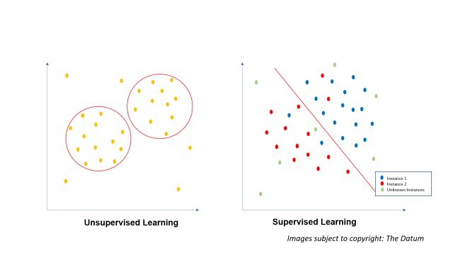
Notional Visuals: Unsupervised vs Supervised Machine Learning
3.2 Unsupervised Learning Algorithm
Clustering is one of the methods of Unsupervised Learning Algorithm: Here we observe the data and try to relate each data with the data similar to its characteristics, thus forming clusters. These clusters hold up a similar type of data which is distinct to another cluster. For example, a cluster of people liking jazz music is distinct from the cluster of people enjoying pop music. This work will help you gain knowledge of one of the of clustering method namely: hierarchical clustering.
Hierarchical Clustering: As the name describes, clustering is done on the basis of hierarchy (by mapping dendrogram: explained further in a practical example of this work)
2. Hierarchical Clustering: Approach
4.1 Density and Distances
Clustering from early stages was developed on the basis of these two instances i.e. Density and Distance. Let us understand each of them:
Density: Goes with the name clearly, if you have a denser data in a particular plane and another dense data in the same plane but at a distance is what known as density clusters on data.
Distance: Two distinct clusters or even data to be a part of cluster 1 or cluster 2 depend upon the separation distance between the two. The distance in Data Science can be computed on the basis of Euclidean distance, Manhattan (City Block) distance, Hamming distance, Cosine distance. These distances are the basics and easy algebraic and geometric understanding. Can be easily refreshed if you are not well versed with them by going back to basics. The figure below illustrates Density and Distance and how it brings clustering, there are two types of data both having a specific density in their respective space, thus they are clustered together as both clusters have distinct characteristics based upon the data they contain. Further, there is also a distance between the two clusters, these distances can be between the individual datums or considering clusters as a whole.
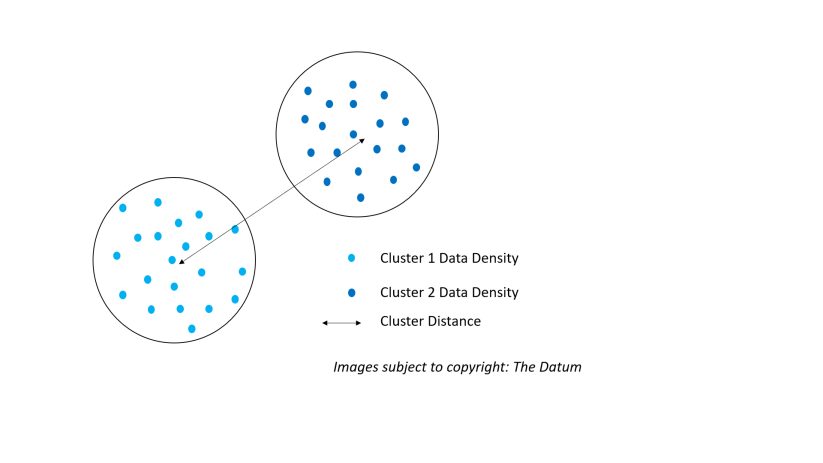
Notional Illustration of Density and Distance in Hierarchical Clustering
4.2 Implementing Hierarchical Clustering in R
4.2.1 The Model Data:
I have used R language to code for clustering on the World Health Organization (WHO) data, containing 35 countries limited to the region of ‘America’[3]. Following are the data fields:
- $Country: contains names of the countries of region America (datatype: string)
- $Population: contains population count of respective countries (datatype: integer)
- $Under15: count of population under 15 years of age (datatype: number)
- $Over60: count of population over 60 years of age (datatype: number)
- $FertilityRate: fertility rate of the respective countries (datatype: number)
- $LifeExpectancy: Life expectancy of people of respective countries (datatype: integer)
- $CellularSubscribers: Count of people of respective countries possessing cellular subscriptions (datatype: number)
- $LiteracyRate: Rate of Literacy of respective countries (datatype: number)
- $GNI: Gross National Income of respective countries (datatype: number)
4.2.2. Setting Goals and Expectations:
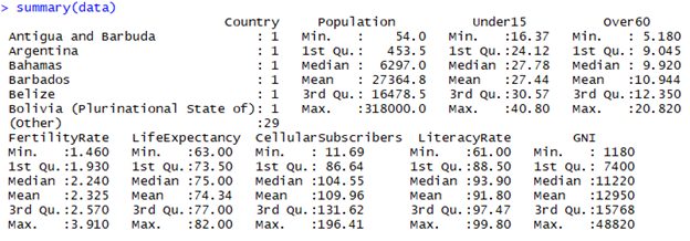
The goal here is to group countries in terms of their health using data fields mentioned above. The data is loaded in R as ‘data’ object and the next image shows the R generated a summary of our data:
 >
>
Summary of Data generated in R
4.2.3 Data Preparation
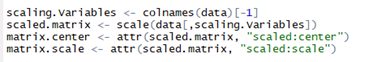
Here, it becomes important that we have all the data fields which are scaled in a disciplined way. This can be considered as the biggest trick to getting your clusters right. If the data is not scaled in the same way, we will not get those distances right and eventually very low confident and bad clusters generation. Scaling the data will form a discipline in all the data field and thus easing our tasks of generating distances. Here I am using scale() function of R to scale the data for mean as 0 and standard deviation of 1 for all the data field except first i.e. $Country. Scale function generates two attributes ‘scaled: center’ and ‘scaled: scale’. Both are then saved in different objects. They can be used again if required to normalize data back again. The below image shows the codes for the same:
 />
/>
Listing for scaling the data
4.2.4. Hierarchical Clustering
To compute hierarchical clustering, I first compute distances using R’s dist() function, to compute distance I have used Euclidean distance, but other distances like Manhattan can also be used. For categorical variables, one might use method=” binary” so as to compute Hamming distance. After having the distance object defined, now I use hclust() function to compute hierarchical clusters using ‘ward.D2’ method. Ward’s[2] method is the classic method to compute such clusters as it starts with individual data points and merges other data points to form a cluster on iterations, this approach of Ward helps minimize total within the sum of squares (WSS) of the clustering. The figures below show the cluster model and dendrogram of the generated clusters and cluster groups.
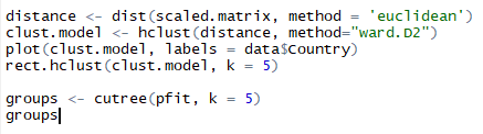
Listings of computing hierarchical model

Groups formed in the model
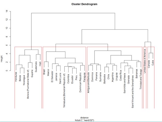
Dendrogram generated by Hierarchical model
Further, we can print the clusters by forming functions to paste the clusters from cutree groups formed. Below shows the listings and printed clusters
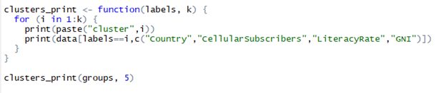
Listings for printing clusters formed
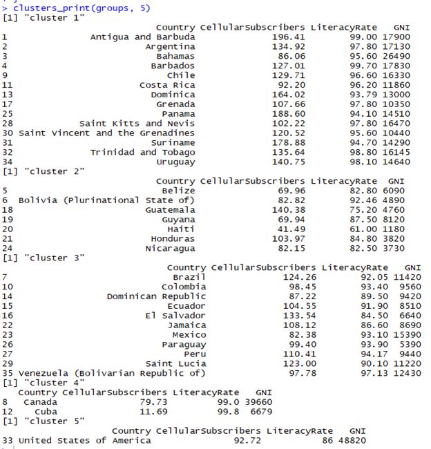
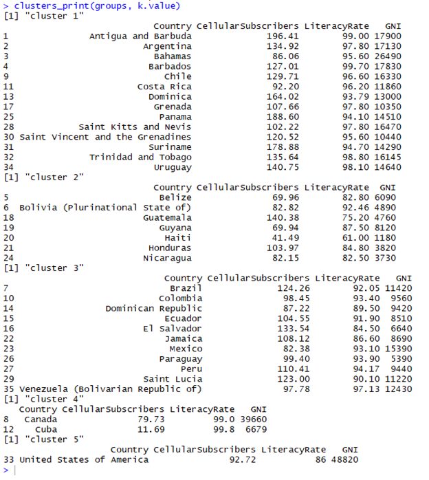
Clusters formed by Hierarchical Clustering
The above information can be interpreted as follows:
- Clusters groups are formed with some similarity geographical areas (with minor trade-offs) into consideration.
- Cluster 1 has high literacy rate with minimum and maximum of being 94.10 and 99.0 respectively
- Cluster 2 has dropped literacy rates with minimum being 61.0 and maximum being 92.46, also they have lowest GNI amongst all the cluster groups
- Cluster 3 has literacy rates around 90’s but not as widely separated as cluster 2
- Cluster 4 has highest literacy rates minimum being 99
- Cluster 5 United States stands alone mainly because of the fact of the varied numbers compared to all other countries in American Region and also, to consider highest GNI amongst all of the countries of $48,820
Interpreting cluster outputs is also about perception, what you can see maybe I cannot and vice-versa. It is always good to spend some time and bring out as much insights as possible.
4.2.5. Visualizing Clusters
In this section, I am going to show you how you can visualize the clusters that are been formed above using R’s ggplot2 library. Clustering visualization can be done using any of the two principal components, remember visualizing a cluster in the first two principal components will show you most of the useful information. This is because, if you have N number of variables in your data, the principal components describe the hyper-ellipsoid space in N-space that bound the data. You are likely to address all the major data variations possible on your data in this space captured in 2 Dimension. Thus, I am using the first 2 principal components, I am calling R’s prcomp() function which will help me do decomposition of principal components. Below are the listing and the later shows the obtained plot.
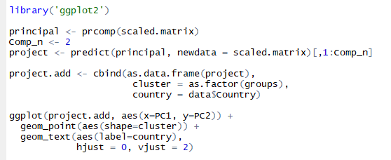
Listing for plotting clusters in first 2 principal components
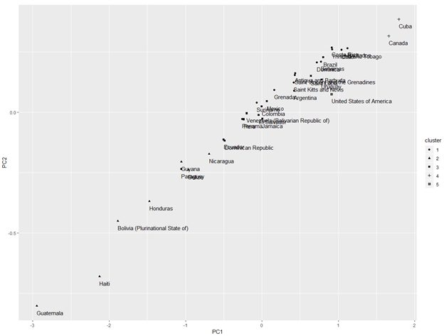
Visualizing clusters represented in first 2 principal components
From the above we observe:
- Cluster 2 is widely spread and is distinct from the other clusters
- Cluster 4 which has just 2 countries Canada and Cuba has its own space
- Cluster 5 of USA is also distinct but in and around the mingling of other clusters
- Rest 1 and 3 of the clusters co-mingle among themselves
Now we have clustered our data and this is all about unsupervised learning and finding some relation among the individual data so that we can relate and find groups. All down and dusted? But wait, are you sure whether the clusters that are formed are based upon real data relationships? Or is it just a fuss of the clustering algorithm?
4.2.6 Bootstrap evaluation of the clusters
Bootstrapping our clusters is the best way to test our clusters against variations in our dataset. We can bootstrap using function clusterboot() in the R package fpc. clusterboot() possesses an interface with hclust() thus making it possible to evaluate our formed clusters based on re-sampling which helps us evaluate how stable is our given cluster.
J(A,B) = |A intersection B| / |A union B|
The above similarity equation is known as Jaccard Similarity. Jaccard is the basis of functioning of clusterboot(). Jaccard Similarity states ‘similarity between two sets A and B is the ratio of the number of elements in the intersection of A and B over the number of elements in the union of A and B.’
Following are the 4 steps to bootstrap your clusters:
- Cluster the data as usual as I have done above
- Create a new data-set (note: size should be similar), this can be easily done by re-sampling our original WHO data-set with few replacements (same data points replicated more than once, and some included not at all). We now cluster new data-set.
- We now look for the similarities in between our original clusters and the new clusters (gives the maximum Jaccard coefficient). There will be a maximum Jaccard coefficient linked to each cluster which indicates dissolution of cluster. The threshold can be set as 0.5 of the maximum Jaccard coefficient is less than 0.5 the original cluster will be considered as to be dissolved, i.e. it did not show up in new clustering. This tells us that a cluster that’s dissolved frequently is probably not a ‘real’ cluster
- Loop steps 2 and 3 multiple times
Following can be considered as maximum Jaccard coefficients values and indicators for the clusters:
| Maximum Jaccard Coefficient | Indicator (Stability) |
| < 0.6 | Unstable Cluster |
| 0.6 – 0.75 | Average but not trusted |
| >0.85 | Highly Stable |
I am now running clusterboot() on my data. I am going to load fpc package and set the desired number of clsuters as 5 (as this was in our original clustering as well), further I am using clusterboot with its respective arguments to get the clusters. Moving ahead clusters will be printed to get the clusters. Below is the listing and output.
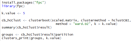
Listing to clusterboot our clusters
Printed clusters from clusterboot (same as original clusters)
Now trust me, if you get this you get a good night’s sleep as a Data Analyst. So, in a nutshell here, I got the same clusters as our original clusters…… exactly same. This shows that our clusters were formed really well to gain high maximum Jaccard coefficients which indicate high stability clusters. Next two more steps, I am going to take this at another level to just verify how exactly stable and useful were our clusters formed. Remember I told you before that each cluster is dissolved for its maximum Jaccard co-efficient? Now I am going to show what you can do to find out a number of dissolutions a cluster went through and each cluster’s maximum Jaccard coefficients. Below is the listing for the same and the output generated.
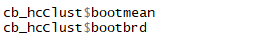
Listing to extract maximum Jaccard coefficients for each cluster and cluster dissolution index (on 100)
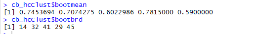
Maximum Jaccard co-efficient and each cluster dissolution (on 100)
The bootmean gives us the maximum Jaccard coefficients, the numbers for our clusters are somewhat acceptable as the are almost all above 0.6 that is above the acceptable stability range.
The bootbrd gives us number of times each cluster was dissolved when clusterboot did 100 times ‘boot’ on each of the clusters.
4.2.7 Are you picking exact K value for your clusters?
For this example illustrated, I visually picked up a number of clusters = 5 just by observing the dendrogram formed, but will you get such easy pickings each time? the answer is no, the real world data is very complex and it will not be the case to visually pick an optimal number of clusters each time. ‘Total within the sum of squares’ and ‘Calinski-Harabasz’ are the two computing algorithms which through computations give us the optimal number of K value for our clusters. This is not listed in this document but it is always good to know things.
3. Conclusion
Hierarchical clustering is the best of the modeling algorithm in Unsupervised Machine learning. The key takeaway is the basic approach in model implementation and how you can bootstrap your implemented model so that you can confidently gamble upon your findings for its practical use. Remember the following:
- Prepare your data by scaling it to the mean value of 0 and standard deviation of 1
- Implement clustering and print/visualize the clusters
- Bootstrap your clusters for testing cluster model confidence
Cheers,
Neeraj