

Every Data Scientist knows that Pandas and NumPy are very powerful libraries, due its capabilities and flexibilities. In this article, we’re going to advanced concepts discuss in detail and how to utilize the same during Data Science implementation.
This article would really help you all during Data Processing/Data Analytics in the Data Science/Machine Learning projects.
Every Data Scientist should be a master those topics to handle the data because data comes from multiple sources and huge files. You supposed to bring all the required data into one place and arrange them physically for your data analysis and visualization point of view. In this regard, we are going to discuss few advanced concepts with effective steps.
Let’s Start!

Let’s starts with Pandas,
pandas offering excellent features as below mentioned in the picture.
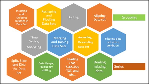
Panel + Data = Pandas
- It provides well-defined data structures and their functions.
- It translates complex operations by using simple commands.
- Easy to group, filtering, concatenating data,
- Well, organized way of doing time-series functionality.
- Sorting, Aggregations, Indexing and re-indexing, and Iterations.
- Reshape the data and its structure,
- Quick slice, and dice the data based on our necessity.
- It translates complex operations by using simple commands.
- Time is taken for executing the commands very fast and expensive.
- Data manipulation capabilities are very similar to SQL.
- Handling data for various aspects like missing data, cleaning, and manipulating data is with a simple line of code.
- Since it has very powerful it can handle Tabular data, Ordered and Unordered time series data, and fit for Un-labelled data.
Why don’t we go through few capabilities from the codebase, so that you could understand better.
Series and DataFrame
Series and DataFrame are the primary Data Structures components of pandas. Series is a kind of dictionary and collection of series, if you merging the series, we could construct the dataframe. Data Frame is a structured dataset, and you can play with that.
- Series
- One Dimensional Array with Fixed Length.
- DataFrame
- Two-Dimensional Array
- Fixed Length
- Rectangular table of data (Column and Rows)
Building Series
import pandas as pd
series_dict={1:’Apple’,2:’Ball’,3:’Cat’,4:’Dall’}
series_obj=pd.Series(series_dict)
series_obj
Output
1 Apple
2 Ball
3 Cat
4 Dall
dtype: object
Building Pandas
import pandas as pd
Eno=[100, 101,102, 103, 104,105]
Empname= [Raja, Babu, Kumar,Karthik,Rajesh,xxxxx]
Eno_Series = pd.Series(Eno)
Empname_Series = pd.Series(Empname)
df = { Eno: Eno_Series, Empname: Empname_Series }
employee = pd.DataFrame(df)
employee
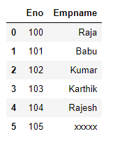
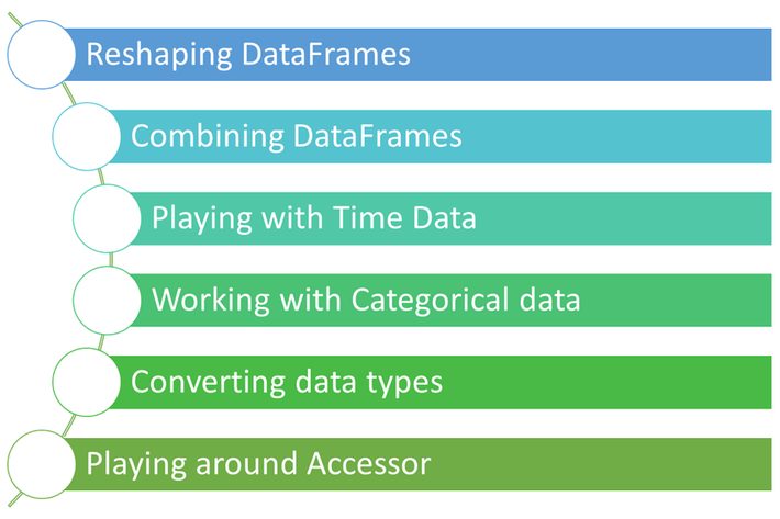
Since we’re targeting “Advanced pandas features”, let’s discuss the below capabilities without wasting the time.
As we know that the pandas is a very powerful library that expedites the data pre-processing stage during the Data Science/Machine Learning life cycle. Below mentioned operations are executed on DataFrame, which represents a tabular form of data with defined rows and columns (We’re clear from the above samples). With this DataFrame only, we use to do much more analytics by applying simple code.
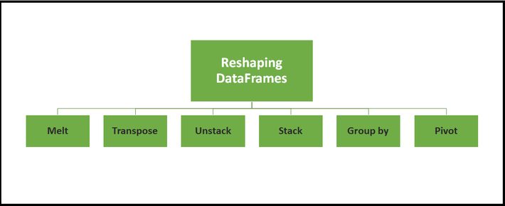
A. Reshaping DataFrames
There are multiple possible ways to reshape the dataframe. Will demonstrate one by one with nice examples.
import pandas as pd
import numpy as np
#building the Dataframe
IPL_Team = {‘Team’: [‘CSK’, ‘RCB’, ‘KKR’, ‘MUMBAI INDIANS’, ‘SRH’,
‘Punjab Kings’, ‘RR’, ‘DELHI CAPITALS’, ‘CSK’, ‘RCB’, ‘KKR’, ‘MUMBAI INDIANS’, ‘SRH’,
‘Punjab Kings’, ‘RR’, ‘DELHI CAPITALS’,’CSK’, ‘RCB’, ‘KKR’, ‘MUMBAI INDIANS’, ‘SRH’,
‘Punjab Kings’, ‘RR’, ‘DELHI CAPITALS’],
‘Year’: [2018,2018,2018,2018,2018,2018,2018,2018,2019,2019,2019,2019,2019,2019,2019,2019,2020,2020,2020,2020,2020,2020,2020,2020],
‘Points’:[23,43,45,65,76,34,23,78,89,76,92,87,50,45,67,89,89,76,92,87,43,24,32,85]}
IPL_Team_df = pd.DataFrame(IPL_Team)
print(IPL_Team_df)
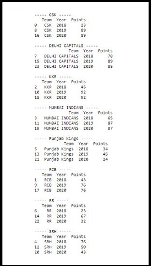
(i)GroupBy
groups_df = IPL_Team_df.groupby(‘Team’)
for Team, group in groups_df:
print(“—– {} —–“.format(Team))
print(group)
print(“”)
Here Groupby feature used to split up DataFrames into multiple groups based on Column.
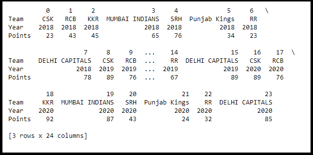
(ii)Transpose
Transposing feature swaps a DataFrames rows with its columns.
IPL_Team__Tran_df=IPL_Team_df.T
IPL_Team__Tran_df.head(3)
#print(IPL_Team__Tran_df)
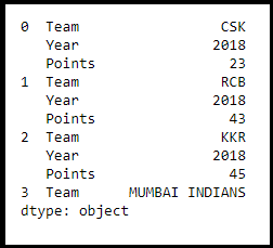
(iii)Stacking
The stacking feature transforms the DataFrame into compressing columns into multi-index rows.
IPL_Team_stack_df = IPL_Team_df.stack()
#print(IPL_Team_stack_df)
IPL_Team_stack_df.head(10)
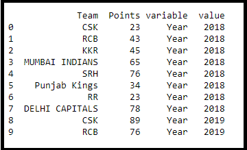
(iv)MELT
Melt transforms a DataFrame from wide format to long format. Melt gives flexibility around how the transformation should take place. In other words, melt allows grabbing columns and transforming them into rows while leaving other columns unchanged (my favourite)
IPL_Team_df_melt = IPL_Team_df.melt(id_vars =[‘Team’, ‘Points’])
print(IPL_Team_df_melt.head(10))
I believe you all are very familiar with the pivot_table. Let’s move.
B. Combining DataFrames
Combining DataFrames is one of the important features to combine DataFrames for different aspects as listed in the below picture.
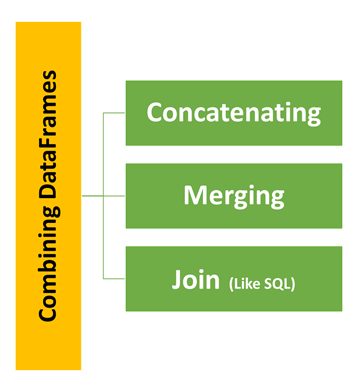
(i)Concatenation
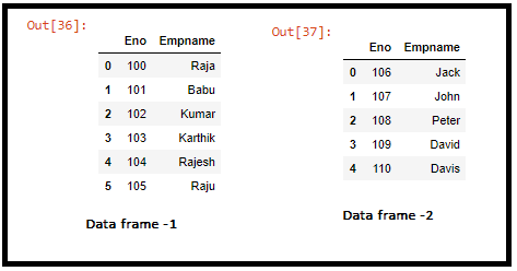
Concatenation is a very simple and straightforward operation on DataFrames, using concat() function along with parameter ignore_index as True. And to identify the sub dataframe from concatenated frames we can use additional parameter keys.
Dataframe -1
import pandas as pd
Eno=[100, 101,102, 103, 104,105]
Empname= [‘Raja’, ‘Babu’, ‘Kumar’,’Karthik’,’Rajesh’,’Raju’]
Eno_Series = pd.Series(Eno)
Empname_Series = pd.Series(Empname)
df = { ‘Eno’: Eno_Series, ‘Empname’: Empname_Series }
employee1 = pd.DataFrame(df)
employee1
Dataframe -2
Eno1=[106, 107,108, 109, 110]
Empname1= [‘Jack’, ‘John’, ‘Peter’,’David’,’Davis’]
Eno_Series1 = pd.Series(Eno1)
Empname_Series1 = pd.Series(Empname1)
df = { ‘Eno’: Eno_Series1, ‘Empname’: Empname_Series1 }
employee2 = pd.DataFrame(df)
employee2
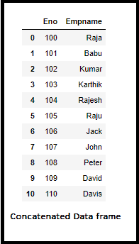
(i-a).Concatenation Operation
df_concat = pd.concat([employee1, employee2], ignore_index=True)
df_concat
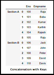
(i-b).Concatination Operation with Key Option
frames_collection = [employee1,employee2]
df_concat_keys = pd.concat(frames_collection, keys=[‘Section-A’, ‘Section-B’])
df_concat_keys
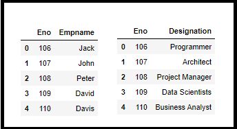
(ii)Merging
We can merge two different DataFrames with different kinds of information and link with some common feature/column. To implement we have to pass dataframe names and additional parameter “on” with the name of the common column.
Dataframe -1
Eno1=[106, 107,108, 109, 110]
Empname1= [‘Jack’, ‘John’, ‘Peter’,’David’,’Davis’]
Eno_Series1 = pd.Series(Eno1)
Empname_Series1 = pd.Series(Empname1)
df = { ‘Eno’: Eno_Series1, ‘Empname’: Empname_Series1 }
employee2 = pd.DataFrame(df)
employee2
Dataframe -2
Eno1=[106, 107,108, 109, 110]
Designation= [‘Programmer’, ‘Architect’, ‘Project Manager’,’Data Scientists’,’Business Analyst’]
Eno_Series1 = pd.Series(Eno1)
Designation_Series1 = pd.Series(Designation)
df = { ‘Eno’: Eno_Series1, ‘Designation’: Designation_Series1 }
Designation_df = pd.DataFrame(df)
Designation_df
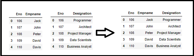
df_merge_columns = pd.merge(employee2, Designation_df, on=’Eno’)
df_merge_columns
Similar to SQL even in the Merge feature as well come up with different options like Outer Join, Left Join, Right Join with parameter how=” join type” will see all these options now.
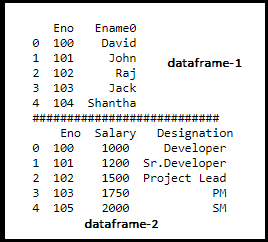
Defining two dataframes
df1 = pd.DataFrame({‘Eno’: [100,101,102,103,104],’Ename0′: [‘David’, ‘John’, ‘Raj’, ‘Jack’,’Shantha’]})
df2 = pd.DataFrame({‘Eno’: [100,101,102,103,105],’Salary’: [1000, 1200, 1500, 1750,2000],
‘Designation’: [‘Developer’, ‘Sr.Developer’, ‘Project Lead’, ‘PM’,’SM’]})
print(df1,”\n###########################\n”,df2)
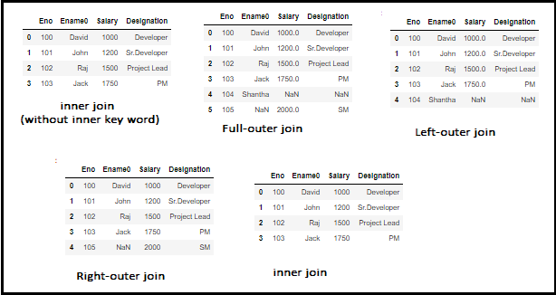
(I)Merging two dataframe using common data with common column available in both dataframe
df_join = pd.merge(df1, df2, left_on=’Eno’, right_on=’Eno’)
df_join
(ii) Full Outer-join
df_outer = pd.merge(df1, df2, on=’Eno’, how=’outer’)
df_outer
(iii)Left-Outer-join
df_left = pd.merge(df1, df2, on=’Eno’, how=’left’)
df_left
(iv)Right-Outer-join
df_right = pd.merge(df1, df2, on=’Eno’, how=’right’)
df_right
(v)Inner-join
df_inner = pd.merge(df1, df2, on=’Eno’, how=’inner’)
df_inner
with JOIN feature which is available under Combining DataFrames.
Note: Even we can merge the dataframe by specifying left_on and right_on columns to merging the dataframe.
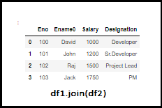
C.JOIN
As mentioned above JOIN is very similar to the Merge option. By default, .join() will do left join on indices.
df1 = pd.DataFrame({‘Eno’: [100,101,102,103],
‘Ename0’: [‘David’, ‘John’, ‘Raj’, ‘Jack’]},
index = [‘0’, ‘1’, ‘2’, ‘3’])
df2 = pd.DataFrame({‘Salary’: [1000, 1200, 1500, 1750],
‘Designation’: [‘Developer’, ‘Sr.Developer’, ‘Project Lead’, ‘PM’]},
index = [‘0’, ‘1’, ‘2’, ‘3’])
df1.join(df2)
Hope we learned so many things, very useful for you everyone, and have to go long way, Here I am passing and continue in my next article(s). Thanks for your time and reading this, Kindly leave your comments. Will connect shortly!
Until then Bye and see you soon – Cheers! Shanthababu.
)