
The Ugly Truth Behind All That Data
We are in the age of data. In recent years, many companies have already started collecting large amounts of data about their business. On the other hand, many companies are just starting now. If you are working in one of these companies, you might be wondering what can be done with all that data.
What about using the data to train a supervised machine learning (ML) algorithm? The ML algorithm could perform the same classification task a human would, just so much faster! It could reduce cost and inefficiencies. It could work on your blended data, like images, text documents, and just simple numbers. It could do all those things and even get you that edge over the competition.
However, before you can train any decent supervised model, you need ground truth data. Usually, supervised ML models are trained on old data records that are already somehow labeled. The trained models are then applied to run label predictions on new data. And this is the ugly truth: Before proceeding with any model training, any classification problem definition, or any further enthusiasm in gathering data, you need a sufficiently large set of correctly labeled data records to describe your problem. And data labeling — especially in a sufficiently large amount — is … expensive.
By now, you will have quickly done the math and realized how much money or time (or both) it would actually take to manually label all the data. Some data are relatively easy to label and require little domain knowledge and expertise. But they still require lots of time from less qualified labelers. Other data require very precise (and expensive) expertise of that industry domain, likely involving months of work, expensive software, and finally, some complex bureaucracy to make the data accessible to the domain experts. The problem moves from merely expensive to prohibitively expensive. As do your dreams of using your company data to train a supervised machine learning model.
Unless you did some research and came across a concept called “active learning,” a special instance of machine learning that might be of help to solve your label scarcity problem.
What Is Active Learning?
Active learning is a procedure to manually label just a subset of the available data and infer the remaining labels automatically using a machine learning model.
The selected machine learning model is trained on the available, manually labeled data and then applied to the remaining data to automatically define their labels. The quality of the model is evaluated on a test set that has been extracted from the available labeled data. If the model quality is deemed sufficiently accurate, the inferred class labels extended to the unlabeled data are accepted. Otherwise, an additional subset of new data is extracted, manually labeled, and the model retrained. Since the initial subset of labeled data might not be enough to fully train a machine learning model, a few iterations of this manual labeling step might be required. At each iteration, a new subset of data to be manually labeled needs to be identified.
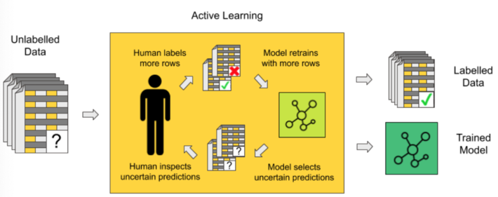
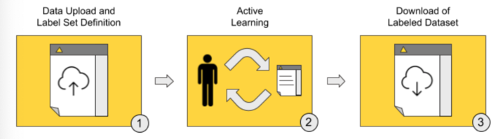
As in human-in-the-loop analytics, active learning is about adding the human to label data manually between different iterations of the model training process (Fig. 1). Here, human and model each take turns in classifying, i.e., labeling, unlabeled instances of the data, repeating the following steps.
Step a –Manual labeling of a subset of data
At the beginning of each iteration, a new subset of data is labeled manually. The user needs to inspect the data and understand them. This can be facilitated by proper data visualization.
Step b –Model training and evaluation
Next, the model is retrained on the entire set of available labels. The trained model is then applied to predict the labels of all remaining unlabeled data points. The accuracy of the model is computed via averaging over a cross-validation loop on the same training set. In the beginning, the accuracy value might oscillate considerably as the model is still learning based on only a few data points. When the accuracy stabilizes around a value higher than the frequency of the most frequent class and the accuracy value no longer increases — no matter how many more data records are labeled — then this active learning procedure can stop.
Step c –Data sampling
Let’s see now how, at each iteration, another subset of data is extracted for manual labeling. There are different ways to perform this step (query-by-committee, expected model change, expected error reduction, etc.), however, the simplest and most popular strategy is uncertainty sampling.
This technique is based on the following concept: Human input is fundamental when the model is uncertain. This situation of uncertainty occurs when the model is facing an unseen scenario where none of the known patterns match. This is where labeling help from a human — the user — can change the game. Not only does this provide additional labels, but it provides labels for data the model has never seen. When performing uncertainty sampling, the model might need help at the start of the procedure to classify even simple cases, as the model is still learning the basics and has a lot of uncertainty. However, after some iterations, the model will need human input only for statistically more rare and complex cases.
After this step c, we always start again from the beginning, step a. This sequence of steps will take place until the user decides to stop. This usually happens when the model cannot be improved by adding more labels.
Why do we need such a complex procedure as active learning?
Well, the short answer is: to save time and money. The alternative would probably be to hire more people and label the entire dataset manually. In comparison, labeling instances using an active learning approach is, of course, more efficient.
Uncertainty Sampling
Let’s have a closer look now at the uncertainty sampling procedure.
As for a good student, it is more useful to clarify what is unclear rather than repeating what the student has already assimilated. Similarly, it is more useful to add manual labels to the data that the model cannot classify confidently than to the data where the model is already confident.
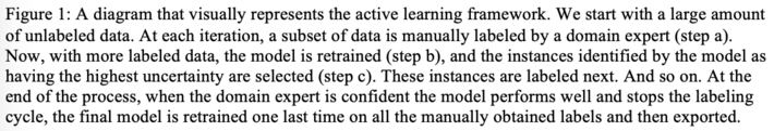
Data where the model outputs different labels with comparable probabilities are the data about which the model is uncertain. For example, in a binary classification problem, the most uncertain instances are those with a classification probability of around 50% for both classes. In a multi-classification problem, highest uncertainty predictions happen when all class probabilities are close. This can be measured via the entropy formula from information theory or, better yet, a normalized version of the entropy score.
![]()
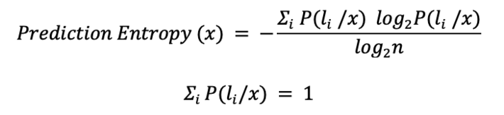
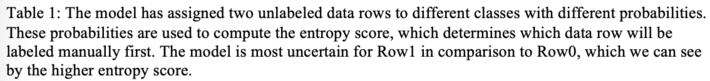
Let’s consider two different data rows feeding a 3-class classification model. The first row was predicted to belong to class 1 (label 1) with 90% probability and to class 2 and class 3 with only 5% probability. The prediction here is clear: label 1. The second data row, however, has been assigned a probability of belonging to all three labels of 33%. Here the class attribution is more complicated.
Let’s measure their entropy. Data in Row1 has a higher entropy value than data in Row0 (Table 1), and this is not surprising. This selection via entropy score can work with any number n of classes. The only requirement is that the sum of the model probabilities always adds up to 1.
Summarizing, a good active learning system should extract all those rows for manual labeling that will benefit most from human expertise rather than more obvious scenarios. After a few iterations, the human-in-the-loop should find the selection of data rows for labeling less random and more unique.
Active Learning as a Guided Labeling Web Application
In this section, we would like to describe a preconfigured and free blueprint web application that implements the active learning procedure on text documents, using KNIME software and involving human labeling between one iteration and the next. Since it takes advantage of the Guifed Analytics feature, it was named “Guided Labeling”.
The application offers a default dataset of movie reviews from Kaggle. For this article, we focus on a sentiment analysis task on this default dataset. The set of labels is therefore quite simple and includes only two: “good” and “bad.”
The Guided Labeling application consists of three stages (Fig. 2).
- Data upload and label set definition. The user, our “human-in-the-loop,” starts the application and uploads the whole dataset of documents to be labeled and the set of labels to be applied (the ontology).
- Active learning. This stage implements the active learning loop.
- Iteration after iteration, the user manually labels a subset of uncertain data rows.
- The selected machine learning model is subsequently trained and evaluated on the remaining subset of labeled data. The increase in model accuracy is monitored until it stabilizes and/or stops increasing.
- If the model quality is deemed not yet sufficient, a new subset of data containing the most uncertain predictions is extracted for the next round of manual labeling via uncertainty sampling.
- Download of labeled dataset. Once it is decided that the model quality is sufficient, the whole labeled dataset — with labels by both human and model — is exported. The model is retrained one last time on all available instances, used to score documents that are still unlabeled, and is then made available for download for future deployments.
![]()
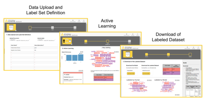
From an end user’s perspective, these three stages translate to the following sequence of web pages (Fig. 3).
![]()
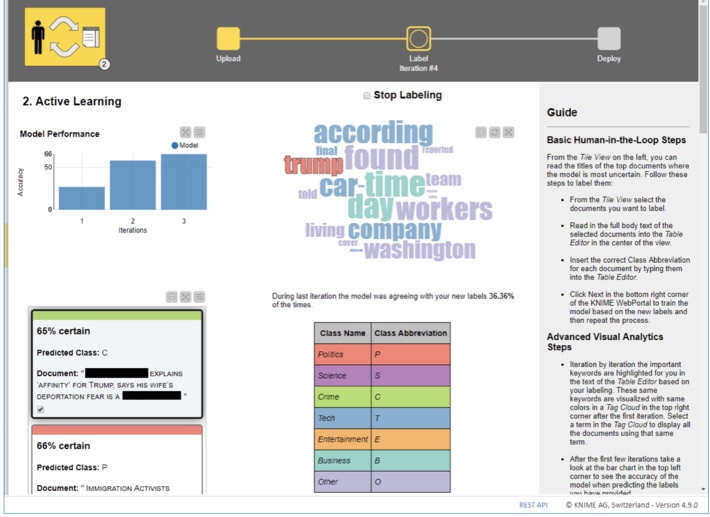
In the first page, the end user has the possibility to upload the dataset and define the label set. The second page is an easy user interface for the quick manual labeling of the data subset from uncertainty sampling.
Notice that this second page can display a tag cloud of terms representative of the different classes. Tag clouds are a visualization used to quickly show the relevant terms in a long text that would be too cumbersome to read in full. We can use the terms in the tag cloud to quickly index documents that are likely to be labeled with the same class. Words are extracted from manually labeled documents belonging to the same class. The top most frequent 50 terms across classes are selected. Of those 50 terms, only the terms present in the still unlabeled documents are displayed in an interactive tag cloud and color coded depending on the document class.
There are two labeling options here:
- Label the uncertain documents one by one as they are presented in decreasing order of uncertainty. This is the classic way to proceed with labeling in an active learning cycle.
- Select one of the words in the tag cloud and proceed with labeling the related documents. This second option, while less traditional, allows the end user to save time. Let’s take the example of a sentiment analysis task: By selecting one “positive” word in the tag cloud, mostly “positive” reviews will surface in the list, and therefore, the labeling is quicker.
Note. This Guided Labeling application works only with text documents. However, this same three-stage approach can be applied to other data types too, for example, images or numerical tabular data.
Guided Labeling in Detail
Let’s check these three stages one by one from the end user point of view.
Stage 1: Data Upload and Label Set Definition
![]()
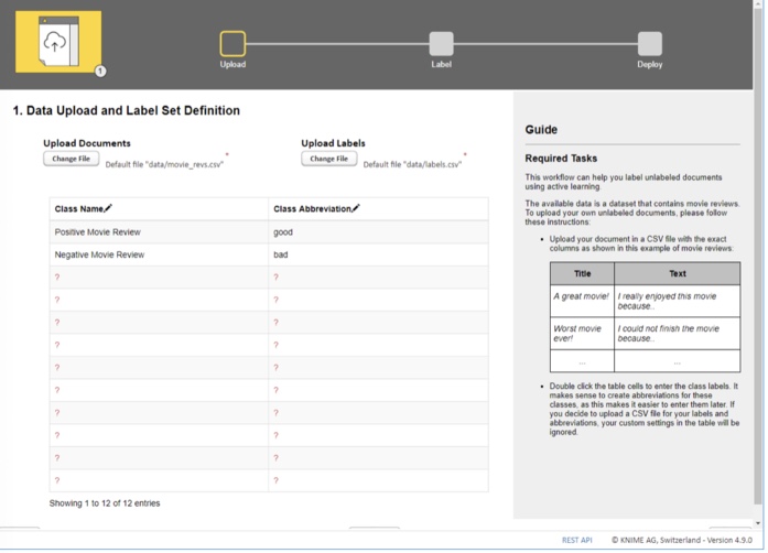
The first stage is the simplest of the three, but this does not make it less important. It consists of two parts (Fig. 4):
- uploading a CSV file containing text documents with only two features: “Title” and “Text.”
- defining the set of classes, e.g., “sick” and “healthy” for text diagnosis of medical records or “fake” and “real” for news articles. If too many possible classes exist we can upload a CSV file listing all the possible string values the label can assume.
Stage 2: Active Learning
It is now time to start the iterative manual labeling process.
To perform active learning, we need to complete three steps, just like in the diagram at the beginning of the article (Fig. 1).
Step 2a –Manual labeling of a subset of data
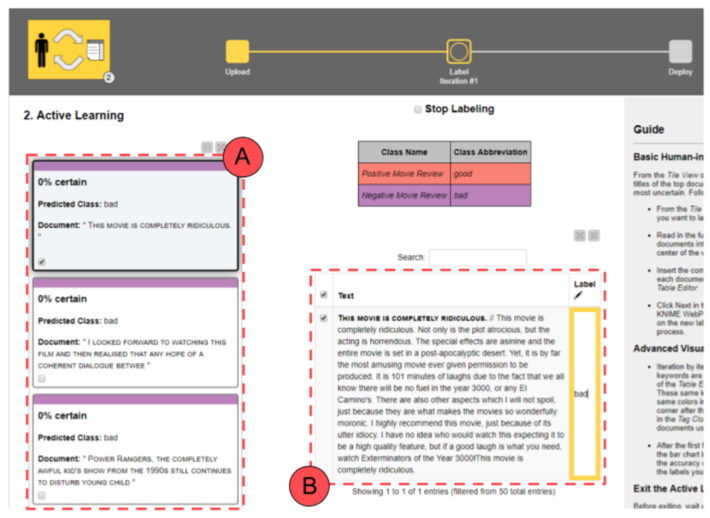
The subset of data to be labeled is extracted randomly and presented on the left side (Fig. 5.1 A) as a list of documents.
If this is the first iteration, no tag clouds are displayed, since no classes have been attributed. Let’s go ahead and, one after the other, select, read and label all documents as “good” or “bad” according to their sentiment (Fig. 5.1 B).
The legend displayed in the center shows the colors and labels to use. Only labeled documents will be saved and passed to the next model training phase. So, if a typo is detected or a document was skipped, this will not be included in the training set and will not affect our model. Once we are done with the manual labeling, we can click “Next” at the bottom to start the next step and move to the next iteration.
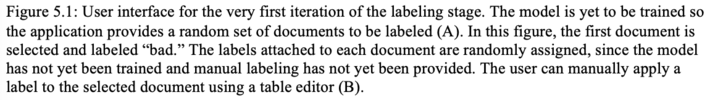
If this is not the first iteration anymore and if the selected machine learning model has already been trained, a tag cloud is created from the already labeled documents. The tag cloud can be used as a shortcut to search for meaningful documents to be labeled. By selecting a word, all those documents containing that word are listed. For example, the user can select the word “awful” in the word cloud and then go through all the related documents. They are all likely to be in need of a “bad” label (Fig 5.2)!
Step 2b –Training and evaluating an XGBoost model
Based on a subset of the few labeled documents to be used as a training set, an XGBoost model is trained to predict the sentiment of the documents. The model is also evaluated on the same labeled data. Finally, the model is applied to all data to produce a label prediction for each review document.
After labeling several documents, the user can see the accuracy of the model improving in a bar chart. When accuracy reaches the desired performance, the user can check the check box “Stop Labeling” at the top of the page, then hit the “Next” button and get to the application’s landing page.
Step 2c –Data sampling
Based on the model predictions, the entropy scorer is calculated for all yet unlabeled data rows; uncertainty sampling is applied to extract the best subset for the next phase of manual labeling. The whole procedure then restarts from step 2a.
![]()
Stage 3: Download of Labeled Dataset
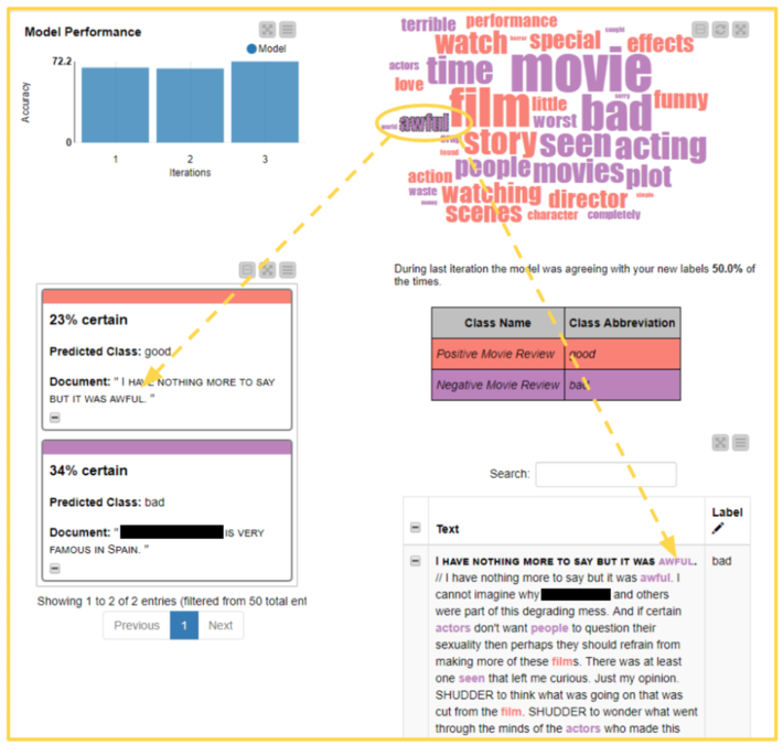
We reached the end of the application. The end user can now download the labeled dataset, with both human and machine labels, and the model trained to label the dataset.
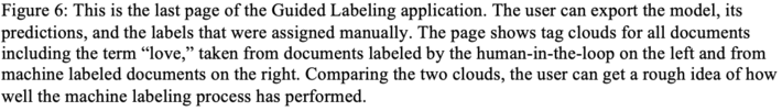
Two word clouds are made available for comparison: on the right, the word cloud of those documents labeled by the human in the loop and on the left, the word cloud of machine labeled documents. In both clouds, words are color coded by document label: red for “good” and purple for “bad.” If the model is performing a decent job at labeling new instances, the two word clouds should be similar and most words in them should have the same color (Fig. 6).
Guided Labeling for Active Learning
In this article, we wanted to illustrate how active learning can be used to label a full dataset while investing only a fractional amount of time in manual labeling. The idea of active learning is that we train a machine learning model well enough to be able to delegate it to the boring and expensive task of data labeling.
We have shown the three stages involved in an active learning procedure: manual labeling, model training and evaluation, and sampling more data to be labeled. We have also shown how to implement the corresponding user interface on a web-based application, including a few tricks to speed up the manual labeling effort using uncertainty sampling.
The example used in this article referred to a sentiment analysis task with just two classes (“good” and “bad”) on movie review documents. However, it could easily be extended to other tasks by changing the number and type of classes. For example, it could be used for topic detection for text documents if we provided a topic-based ontology of possible labels (Fig. 7). It could also be extended just as simply to other data types and classification tasks.
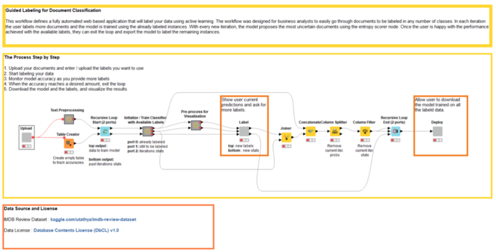
The Guided Labeling application was developed via a KNIME workflow (Fig. 8) It is now your turn to try out the Guided Labeling application yourself. See how easily and quickly data labeling can be done!
![]()

Paolo Tamagnini contributed to this article. He is a data scientist at KNIME, holds a master’s degree in data science from Sapienza University of Rome and has research experience from NYU in data visualization techniques for machine learning interpretability. Follow Paolo on LinkedIn.