
In part 1 of this article series, I provided a quick primer on graph data structure, acknowledged that there are several graph based algorithms with the notable ones being the shortest path/distance algorithms and finally illustrated Dijkstra’s and Bellman-Ford algorithms. Continuing with the shortest path/distance algorithms, I have illustrated Floyd-Warshall and A* (A-Star) algorithms in this part 2 of the article. As was stated in part 1, while the inner workings of these algorithms are thoroughly covered in many text books and informative resources online, I felt that not many provided visual examples that would otherwise illustrate the processing steps to sufficient granularity enabling easy understanding of the working details. In addition, a solid understanding of the intuition behind such algorithms not only helps in appreciating the logic behind them but also helps in making conscious decisions about their applicability in real life cases.
Floyd-Warshall’s Algorithm
Floyd-Warshall’s algorithm is a dynamic programming based algorithm to compute the shortest distances between every pair of the vertices in a weighted graph where negative weights are allowed. Dynamic programming is a problem-solving approach in which a complex problem is incrementally solved, essentially iteratively, in a way that the values computed in previous iteration are used to compute the values in the current iteration. As such, to qualify for dynamic programming, a problem should be divisible into sub-problems with identical problem context. Floyd-Warshall employs dynamic programming approach by dividing a path between two vertices into two sub-paths that are connected via a third intermediary vertex. For example, a path between vertices A and D can be considered as a path via a third intermediary vertex C so that distance d(A,D) can be computed as sum of distances d(A,C) and d(C,D), i.e., d(A,D) = d(A,C) + d(C,D) and then the path between vertices A and C can be further considered as a path via yet another intermediary vertex B so that d(A,C) = d(A,B) + d(B,C). As such, the main problem of computing distance between vertices is divided into sub-problems of computing intermediary distances wherein both the main problem and the sub-problems deal with the identical context of finding distances between two vertices. At every step in the dynamic programming approach, Floyd-Warshall algorithm determines a shortest tentative distance between two vertices. Note that a distance between two vertices is considered as tentative until algorithm confirms it to be the shortest distance. The core of the algorithm is that the shortest distance between vertices A and C is minimal of either the tentative shortest distance found so far between A and C or the sum of the tentative shortest distances from A to B and from B to C, where B is the intermediate vertex. The algorithm iterates over the vertices of the graph and at each iteration, treats current iteration vertex as the intermediary while evaluating the tentative distances between pairs of other vertices. The algorithm completes after testing every pair possible in the graph and every intermediate vertex possible between a pair.
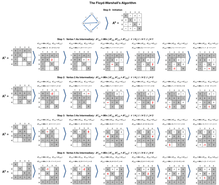 Figure 3 : Illustrations of Floyd-Warshall Algorithm
Figure 3 illustrates the logical steps in the execution of Floyd-Warshall algorithm. In essence, the algorithm maintains an adjacency matrix comprising of evaluated distances between every pair of vertices that would get updated at each iteration. The example graph contains 4 vertices and hence algorithm would maintain an adjacent matrix of size 4 x 4 = 16 values. As an example, the value in 3rd row and 2nd column represents the evaluated distance between vertex 3 and vertex 2. At step 0, the algorithm initiates the matrix values. The algorithm sets distance of a vertex to itself as 0 as shown in the diagonal values of the matrix. The algorithm sets known direct edge weights between any two vertices as initial distances in the matrix. For all other pairs of vertices without direct edges, the algorithm sets the distances as infinity in the matrix.
The algorithm then begins step 1. At step 1, the algorithm employs dynamic programming approach by evaluating the minimum tentative distance between a pair of vertices by treating vertex 1 as the intermediate vertex. As such the algorithm evaluates the tentative distance between vertices i and j, A1( i, j ), as the minimum of either A0( i, j ) or A0( i, 1 ) + A0( 1, j ) for all values of i and j where i is not equal to j and neither i nor j equal to 1. In this case, A1 is the copy of adjacency matrix being updated in step 1 while A0 is the adjacency matrix created at initiation step 0. Essentially the dynamic programming formula of evaluating distances at step 1 is given by A1( i, j ) = Min( A0( i, j ), A0( i, 1 ) + A0( 1, j ) ) ∀ i ≠ j ⋀ i ≠ 1 ⋀ j ≠ 1. Because the formula constraints must be satisfied during the execution, the algorithm fixes the row 1, column 1 and the diagonal values for step 1 as shown in the figure 3. This means that the fixed values cannot be updated during this step. As such, the only distances that can be evaluated in step 1 are A1( 2, 3 ), A1( 2, 4 ), A1( 3, 2 ), A1( 3, 4 ), A1( 4, 2 ) and A1( 4, 3 ). The algorithm would evaluate the value A1( 2, 3 ) using the formula A1( 2, 3 ) = Min( A0( 2, 3 ), A0( 2, 1 ) + A0( 1, 3 ) ). Similarly, algorithm would evaluate the value A1( 4, 3 ) using the formula A1( 4, 3 ) = Min( A0( 4, 3 ), A0( 4, 1 ) + A0( 1, 3 ) ). As illustrated in figure 3 step 1, the algorithm would evaluate and update the values of A1 matrix accordingly to complete step 1.
The algorithm then begins step 2. At this step, the algorithm employs dynamic programming approach by evaluating the minimum tentative distance between a pair of vertices by treating vertex 2 as the intermediate vertex. Essentially the dynamic programming formula of evaluating distances at step 2 is given by A2( i, j ) = Min( A1( i, j ), A1( i, 2 ) + A1( 2, j ) ) ∀ i ≠ j ⋀ i ≠ 2 ⋀ j ≠ 2. In this case, A2 is the copy of adjacency matrix being updated in step 2 while A1 is the copy of adjacency matrix updated in step 1. In this step, the algorithm fixes row 2, column 2 and the diagonal values and hence the distances that can be evaluated in step 2 are A2( 1, 3 ), A2( 1, 4 ), A2( 3, 1 ), A2( 3, 4 ), A2( 4, 1 ) and A2( 4, 3 ). The algorithm would evaluate the value A2( 1, 3 ) using the formula A2( 1, 3 ) = Min( A1( 1, 3 ), A1( 1, 2 ) + A1( 2, 3 ) ). Similarly, the algorithm would evaluate the value A2( 4, 3 ) using the formula A2( 4, 3 ) = Min( A1( 4, 3 ), A1( 4, 2 ) + A1( 2, 3 ) ). Using this approach as shown in figure 3 step 2, the algorithm would evaluate and update the values of A2 matrix and complete step 2. In a similar manner, the algorithm executes step 3 and step 4. Note that at step 3, the algorithm evaluates the minimum tentative distance between a pair of vertices by treating vertex 3 as the intermediate vertex using the dynamic programming formula A3( i, j ) = Min( A2( i, j ), A2( i, 3 ) + A2( 3, j ) ) ∀ i ≠ j ⋀ i ≠ 3 ⋀ j ≠ 3, where A3 is the copy of adjacency matrix being updated in step 3 while A2 is the copy of adjacency matrix updated in step 2. Similarly, at step 4, the algorithm evaluates the minimum tentative distance between a pair of vertices by treating vertex 4 as the intermediate vertex using the dynamic programming formula A4( i, j ) = Min( A3( i, j ), A3( i, 4 ) + A3( 5, j ) ) ∀ i ≠ j ⋀ i ≠ 4 ⋀ j ≠ 4, where A4 is the copy of adjacency matrix being updated in step 4 while A3 is the copy of adjacency matrix updated in step 3. The updated matrix at step 4 contains the final shortest distances between any pair of vertices in the example graph.
As can be inferred from the illustration, the algorithm executes N steps where N is the number of vertices in the graph. At each step, the algorithm evaluates utmost (N2 – 3N + 2) number of tentative distance values. Therefore the total number of distances evaluated by the algorithm is given by N x (N2 – 3N + 2). As such the time complexity of Floyd-Warshall algorithm is in the order of N3. This time complexity is same as if executing Dijkstra’s algorithm (with time complexity of N2) N number of iterations where at each iteration, a vertex in the graph is considered as the source vertex to evaluate its distances to remaining vertices.
A* (A-Star) Algorithm
A* algorithm is a heuristic based, greedy, best-first search algorithm used to find optimal path from a source vertex to a target vertex in a weighted graph. As was stated in part 1, an algorithm is said to be greedy if it leverages local optimal solution at every step in its execution with the expectation that such local optimal solution will ultimately lead to global optimal solution. A* algorithm works on a greedy expectation that a vertex with lowest evaluated cost is the best vertex to be on the path that will lead to the optimal path from the starting vertex to the target vertex. Incremental estimate of cost is evaluated based on two cost components. If V is the next vertex on the path, then the estimate of the cost is given by f(V) = h(V) + g(V), where h(V) is a heuristic associated with vertex V and g(V) is the estimated cost of the path thus far from the source vertex to vertex V. While g(V) is estimated as sum of edge weights from the source vertex to vertex V as in Dijkstra’s algorithm, the value h(V) is an assigned value to vertex V that can be considered as a metric indicating how close vertex V is from the target vertex.
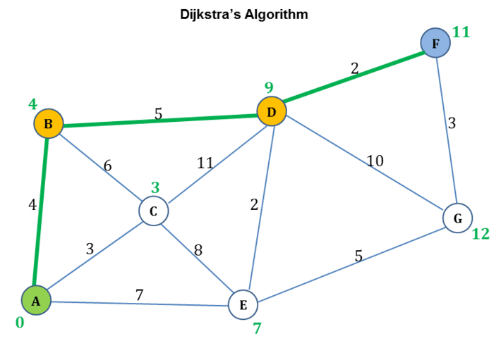 Figure 4 : Dijkstra’s Algorithm Example
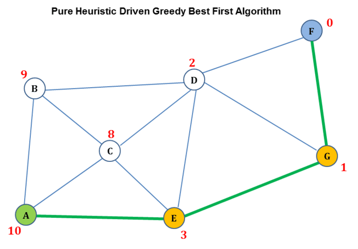
Figure 5 : Pure Greedy Best First Algorithm Example
As was illustrated in part 1 and as shown in figure 4, Dijkstra’s algorithm guarantees a shortest path from a source vertex A to target vertex F, however at the expense of computing shortest paths to every other vertex from source vertex A. Dijkstra’s algorithm greedily selects next vertex on the path purely based on how close the vertex is from the source vertex. Dijkstra’s algorithm does not take into consideration any heuristic indicating how close the next vertex is from the target vertex. The shortest path computed by Dijkstra’s algorithm in the example is {A, B, D, F}. On the other hand, as shown in figure 5, a pure heuristic driven, greedy, best first algorithm goes about picking the next vertex purely based on the vertex’s closeness to the target vertex indicated by the associated heuristic value. It does not take into consideration how close the next vertex is from the source vertex. As shown in figure 5, starting at source vertex A, the algorithm first selects vertex E as the next vertex because it has lower heuristic compared to vertices B and C. Then starting at vertex E, the algorithm selects vertex G as the next vertex because it has lower heuristic compared to vertex D and finally starting at vertex G, the algorithm selects the target vertex F whose heuristic is 0. As such the optimal path computed by pure greedy best first algorithm, in the example, is {A, E, G, F}.
A* can be considered as an algorithm that tries to combine the best of the both worlds – Dijkstra’s and pure greedy best first algorithms. In essence, A* algorithm not only considers how close next vertex is from the target vertex indicated by h(n) but also considers how close next vertex is from the source vertex indicated by g(n) to find the optimal path. Starting at the source vertex, the algorithm would evaluate f(n) = h(n) + g(n) value for all the neighbors and will pick the neighbor V with lowest f(n) value as the next vertex on the path. The algorithm would repeat computing f(n) values for the neighbors of vertex V and selects the next vertex with lowest f(n) value. The algorithm repeats this process until evaluation reaches the target vertex.
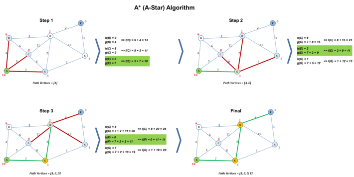 Figure 6 : Illustrations of A* Algorithm
Figure 6 illustrates the logical steps in the execution of A* algorithm. The steps are intentionally simplified to ensure that focus is on understanding the intuition. The goal of the algorithm in the illustration is to find the optimal path between source vertex A and target vertex F. Each vertex in the weighted graph is assigned with a heuristic value relative to target vertex. The algorithm maintains an ordered set representing path vertices, initially containing the source vertex A. As shown in figure 6, at step 1, the algorithm starts at source vertex A and computes f(n) = h(n) + g(n) for each of its neighbors, B, C and E. The algorithm selects vertex E as the next best vertex as its f(n) value 10 is the lowest as compared to B’s value of 13 and C’s value of 11. The algorithm adds vertex E to the path vertices set. At step 2, the algorithm moves to vertex E and computes f(n) value for each of the neighbors of vertex E – value of 23 for vertex C, 11 for vertex D and 13 for vertex G in the example. Since vertex D’s f(n) value is the lowest, the algorithm selects vertex D as the next best and adds it to the path vertices set. The algorithm then moves to vertex D at step 3 and computes f(n) values for its neighbors – a value of 28 for vertex C, 11 for vertex F and 20 for vertex G. The algorithm selects vertex F since it has the lowest f(n) value, adds vertex F to the path vertices set and moves to vertex F. The algorithm determines that it has reached the target vertex F and stops the execution. The resulting path vertices set contains the optimal path {A, E, D, F}.
One of the main challenges in employing A* algorithm is the determination of vertex heuristic values. There are suggested methods to compute either exact values or approximate values, covering whose detail is perhaps a different discussion topic. Whichever method is employed, it is generally suggested that heuristic values assigned to vertices are distinct so that no two vertices get the same heuristic value. This is to avoid the need for breaking a potential tie when more than one vertex ends up getting same f(n) value. The selection of the heuristic computation method also impacts the time complexity of A* algorithm. In the worst case, the time complexity can depend exponentially on the number of vertices for which f(n) value would need to be evaluated.
More Algorithms
In the upcoming continuation parts of this article, I will cover additional graph based shortest path algorithms with concrete illustrations and I hope that such illustrations would help in understanding intuitions behind such algorithms.