
Linear regression uses Ordinary Least square method to find the best coefficient estimates. One of the assumptions of Linear regression is that the variables are not correlated with each other. However, when the multicollinearity exists in the dataset (two or more variables are highly correlated with each other) Ordinary Least square method cannot be that effective. In this blog, we will talk about two methods which are slightly better than Ordinary Least Square method – Lasso and Ridge regression.
Lasso and Ridge regressions are closely related to each other and they are called shrinkage methods. We use Lasso and Ridge regression when we have a huge number of variables in the dataset and when the variables are highly correlated.
Before we jump onto the intuition behind Lasso and Ridge regression let us understand why we implement these regressions in the first place.
Bias-Variance Trade-off
We know that the Linear regression is given by below equation:
Y = XT * β + ε, ε (0, σ2)
Where ε is the error which is normally distributed.
In regression, our main goal is the find the optimum value of
XT * β
Where X denotes the input variable matrix from the dataset
We know that it is next to impossible to find the exact value of β but we can find the estimated value βᶺ (predicted β) which will be very close to our actual β value.
For the above equation let us consider that we have an estimator given by
XT * βᶺ
In order to verify if we have the optimum value of XT * βᶺ, we check if our predicted value is close to the actual value (XT * β) and how well our function is fitting the new dataset (future dataset).
In order to evaluate this, we consider mean squared error of our estimated βᶺ (predicted value of β)
MSE(βᶺ) = E [| βᶺ – β|2]
Where E is the true expectation (mean)
If our model is performing well on our existing dataset then important factor to consider is that is our model performing well on the new dataset?
In order to evaluate this, we calculate the predicted error which can be explained as the difference between the actual y and the predicted y from the new dataset.
We may estimate a model Yᶺ of Y using linear regression or any other modeling technique. In this case, the expected squared predicted error at a point x is given by:
Err(x) = E [(Y – fᶺ(x))2]
This error can be decomposed into bias and variance as:
Err(x): (E[fᶺ(x)] – f(x))2 + E[(fᶺ(x) – E[fᶺ(x)])2 ] + σ2
Where f(x)= Y
Predicted Error: Bias2+ Variance + Irreducible Error
The irreducible error is the inherent uncertainty around the mean and we cannot do anything about the inherent uncertainty. So, we just have to deal with bias and variance of the model. Dealing with these two errors will help in reducing Mean squared error which in turn will reduce the predicted error of the estimation.
Bias: The bias is an error from erroneous assumptions in the learning algorithm. It simply means how far away is our estimated values from actual values. In the figure below, let’s say our target is the central red circle. If our predictions (blue dots) are close to the original target, then we say we have a low bias. High bias can cause an algorithm to miss the relevant relations between features and target outputs (underfitting).
Variance: The variance is an error from sensitivity to small fluctuations in the training set. It is a measure of spread or variations in our predictions. High variance can cause an algorithm to model the random noise in the training data, rather than the intended outputs (overfitting).
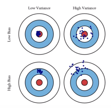
Source: Google images
Let’s say that we have a perfect model where the variables are not correlated to each other (dataset does not exhibit multicollinearity). In this situation, the bias and variance in our model will be very low as depicted in the top left diagram. This means that our predicted value will be very close to the actual value. But as the variance in our model goes on increasing the spread of the prediction will also start increasing which would result in wrong predicted values in the new or test data. That is, the model will have poor generalization power.
The bias-variance curve, sometimes called bias-variance trade-off, with low bias and high variance, will look something like this:
 source: Google images
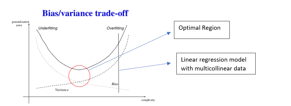
This graph shows how the bias and variance change as the complexity(parameters) of the model increases. As complexity increases, variance increases and bias decreases. For any machine learning model, we need to find a balance between bias and variance to improve generalization capability of the model. This area is marked in the red circle in the graph.
As shown in the graph, Linear Regression with multicollinear data has very high variance but very low bias in the model which results in overfitting. This means that our estimated values are very spread out from the mean and from one another. The model captures the noise and outliers in the dataset along with the underlying patterns which result in overfitting of the data.
Similarly, if we have low variance and high bias in our model then it would result in underfitting of the data. This means that model is unable to find the underlying patterns within the dataset. These models are usually simple models.
In practice, like mentioned above, we would want to have a trade-off between these two error components. As evident from the graph, for Linear Regression with multicollinear data, a small increase in bias can result in a big decrease in the variance and which would result in a substantial decrease in Predicted error. Hence our goal is to move the trade-off line more towards left-hand side.
One of the most common methods to avoid overfitting is by reducing the model complexity using regularization.
When the β coefficients are unconstrained(OLS) they can tend to have high value (in multicollinear cases), which would result in very high variance in the model. In order to control the variance, we add a constraint to the beta coefficients while estimating them. This constraint is nothing but the penalty parameter given by λ (lambda). This type of regression where we add penalty parameter λ in order to estimate the β coefficients is called Ridge and Lasso regression.
Ridge Regression:
Ridge regression is an extension of Linear regression. It is a regularization method which tries to avoid overfitting of data by penalizing large coefficients. Ridge regression has an additional factor called λ (lambda) which is called the penalty factor which is added while estimating beta coefficients. This penalty factor penalizes high value of beta which in turn shrinks beta coefficients thereby reducing the mean squared error and predicted error.
In Linear equation, we simply try to find the values of beta coefficients by minimizing the error without any constraints which will be given by
![]()
However, in Ridge regression, we optimize the Residual Sum Squares subject to a constraint on the sum of squares of the coefficients,
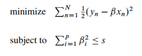
Here, s is constrained value.
The above equation can be further decomposed into below equation:
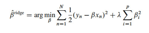
In matrix notation, it can be written as:
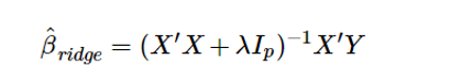
Which is an extension of OLS which we explained in our previous post.
Here, λ value will always be greater than 0 and this parameter controls the amount of shrinkage. This is a parameter we have to choose (tuning parameter). The penalty parameter is applied β1…βp and not to the intercept β0 since it is simply the mean value of the response variable. The value of lambda varies between 0 and ∞ but practically we keep the value between 0 and 1. We want to select the value of lambda such that it minimizes the mean squared error. Cross-validation is often used to select λ where we select the grid of λ values and then compute cross-validation error of each of that λ. We finally select that value of λ which gives the smallest cross-validation predicted error.
When λ = 0, the regression will be similar to linear regression and the β coefficient estimates will be similar to linear regression β coefficients.
Higher the value of λ, greater will be the shrinkage of the β coefficients and this, in turn, makes the coefficients more robust to collinearity. However, the important factor to notice here is that Ridge regression enforces β coefficients to converge to 0 but does not make their value 0. This means that Ridge regression will not enforce the irrelevant variable coefficients to become 0 rather, it will reduce the impact of these variables on the model.
Lasso regression:
Lasso regression is another extension of the linear regression which performs both variable selection and regularization. Just like Ridge Regression Lasso regression also trades off an increase in bias with a decrease in variance. However, Lasso regression goes to an extent where it enforces the β coefficients to become 0.
Lasso regression also follows similar equation like Ridge regression but with a slight change in the equation.
Lasso regression equation is given as:
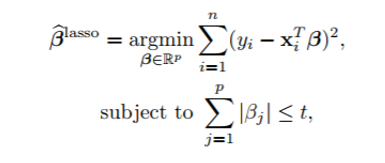
Here, t is the constrained value.
The above equation can be further decomposed into below equation:
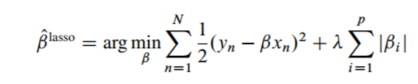
The only difference between lasso and Ridge regression equation is the regularization term is an absolute value for Lasso. The Lasso regression not only penalizes the high β values but it also converges the irrelevant variable coefficients to 0. Therefore, we end up getting fewer variables which in turn has higher advantage.
R code:
One important point before R implementation. Unlike Ordinary Least Squared Regression(OLS), for Lasso and Ridge, we need to standardize the input variable.
We usually standardize variables when two or more independent variables have different scales. We now know that Lasso and ridge regression is nothing but regularization of linear regression where we add penalty parameter to shrink the coefficients and push them more towards 0. If the independent variables are of different scale then penalty parameter will have a different impact on these variable coefficients and this would result in unfair shrinking since the penalized term is nothing but the sum of square of all coefficients. Hence to avoid this problem of unfair shrinking we standardize our input variable matrix in order to have variance 1.
Let us see how Ridge and Lasso performs better than Linear regression
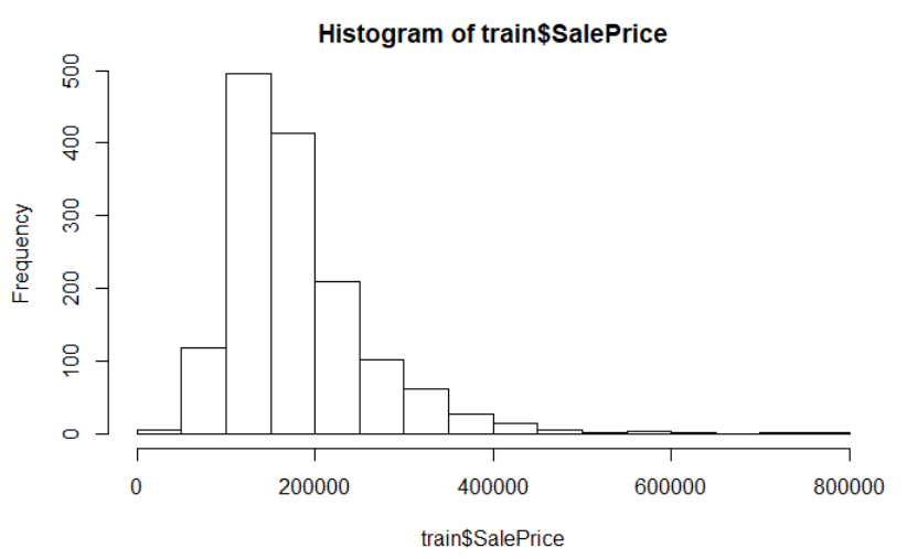
I am using Ames Housing dataset where we have various parameters and our aim is to predict the final price of each house. This dataset is taken from kaggle which can be downloaded here.
After looking at the dataset, I found that the dependent variable is not normally distributed so we follow the standard method to transform this variable using log transformation.
hist(train$SalePrice)
hist(log(train$SalePrice))
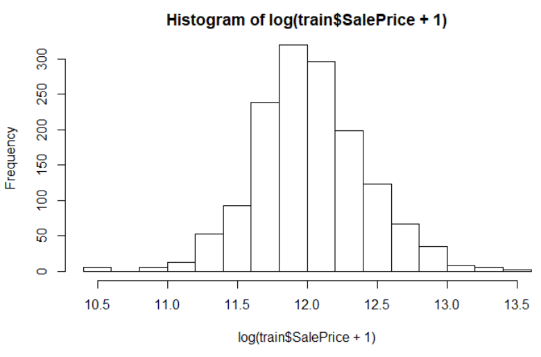
Hence, we perform transformation of dependent variable
train$SalePrice <- log(train$SalePrice)
For numeric features with excessive skewness, we perform log transformation
feature_classes <- sapply(names(train),function(x){class(train[[x]])})
numeric_feats <-names(feature_classes[feature_classes != “character”]) install.packages(“moments”)
library(moments)
skewed_feats <- sapply(numeric_feats,function(x){skewness(train[[x]],na.rm=TRUE)})
keep only features that exceed a threshold for skewness
skewed_feats <- skewed_feats[skewed_feats > 0.75]
Transform excessively skewed features with log(x + 1)
for(x in names(skewed_feats)) {
train[[x]] <- log(train[[x]] + 1)
}
Get names of categorical features
categorical_feats <- names(feature_classes[feature_classes == “character”])
Use caret dummyVars function for hot one encoding for categorical features library(caret)
dummies <- dummyVars(~.,train[categorical_feats])
categorical_1_hot <- predict(dummies,train[categorical_feats])
For any level that was NA, let us set it to zero categorical_1_hot[is.na(categorical_1_hot)] <- 0 numeric_df <- train[numeric_feats]
for (x in numeric_feats) {
mean_value <- mean(train[[x]],na.rm = TRUE)
train[[x]][is.na(train[[x]])] <- mean_value
}
train <- cbind(train[numeric_feats],categorical_1_hot)
x<- subset(train,select= -SalePrice)
y <- train$SalePrice
Now, our dataset is ready for modeling
Setting up caret model training parameters using ‘caret’ package
Model specific training parameter
CARET.TRAIN.CTRL <- trainControl(method=”repeatedcv”,
number=5,
repeats=5,returnResamp=”final”,
verboseIter=FALSE)
Linear Regression
model_linear <- train(SalePrice~.,train,method=”lm”,metric=”RMSE”,maximize=FALSE,trControl=CARET.TRAIN.CTRL)
summary(model_linear)
mean(model_linear$resample$RMSE)
Output: 0.3923876
Ridge Regression
set.seed(123) # for reproducibility
model_ridge <- train(x=x,y=y, method=”glmnet”, metric=”RMSE”,maximize=FALSE,trControl=CARET.TRAIN.CTRL,tuneGrid=expand.grid(alpha=0, lambda=0.039)) #alpha is set to 0 for Ridge regression
mean(model_ridge$resample$RMSE)
Output: 0.1323638
Lasso Regression
set.seed(123) # for reproducibility
model_lasso <- train(x=x,y=y,
method=”glmnet”,
metric=”RMSE”,
maximize=FALSE,
trControl=CARET.TRAIN.CTRL,
tuneGrid=expand.grid(alpha=1,lambda=0.01)) # alpha is set to 1 for Lasso regression
model_lasso
mean(model_lasso$resample$RMSE)
Output: 0.1296652
We can see that Ridge and Lasso is performing far better than Linear Regression when the correlation exists in the dataset. We can tune our penalty parameter further and try to find best value of RMSE. Here, 0.01 is the best value I got for lambda. So, we can use these regression methods when the variables are highly correlated.
Hope this article was useful in understanding Bias-Variance trade-off, Lasso and Ridge Regression. Please feel free to comment, give feedback and share this article if you found it useful.
You can find the original article on my blog here.