This formula-free summary provides a short overview about how PCA (principal component analysis) works for dimension reduction, that is, to select k features (also called variables) among a larger set of n features, with k much smaller than n. This smaller set of k features built with PCA is the best subset of k features, in the sense that it minimizes the variance of the residual noise when fitting data to a linear model. Note that PCA transforms the initial features into new ones, that are linear combinations of the original features. 

Steps for PCA

The PCA algorithm proceeds as follows:

1. Normalize the original features: remove the mean from each  feature
2. Compute the covariance matrix on the normalized data. This is an n x n symmetric matrix, where n is the number of original features, and the element in row i and column j is the covariance between the i-th and j-th column in the data set.  
3. Calculate the eigenvectors and eigenvalues of the covariance matrix. These eigenvectors must be unit eigenvectors, that is, their lengths are 1. This step is the most intricate, and most software packages can do it automatically.
4. Choose the k eigenvectors with the highest eigenvalues.
5. Compute the final k features, associated with the k highest eigenvalues: for each one, multiply the data set matrix, by the associated eigenvector. Here we assume that the eigenvector has one column and n rows (n is the number of original variables), while the data set matrix has n columns and m rows (m is the number of observations), Thus the resulting final features have m rows and one column: it provides the values for the new features, computed at each of the m observations.
6. You may want to put back the mean that was removed in step #1.

The proportion of the variance that each eigenvector represents can be calculated by dividing the eigenvalue corresponding to that eigenvector by the sum of all eigenvalues.

Caveats 

If the original features are highly correlated, the solution will be very unstable. Also the new features are linear combinations of the original features, and thus, may lack interpretation. The data does not need to be multinormal, except if you use this technique for predictive modeling using normal models to compute confidence intervals.

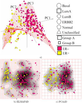Source for picture: click here 

Click here (Wikipedia) to read the implementation details. This is a very long article, but you can focus on the section entitled Computing PCA using the covariance method.

DSC Resources

• Services: Hire a Data Scientist | Search DSC | Classifieds | Find a Job
• Contributors: Post a Blog | Ask a Question
• Follow us: @DataScienceCtrl | @AnalyticBridge

Popular Articles

• Difference between Machine Learning, Data Science, AI, Deep Learnin...
• What is Data Science? 24 Fundamental Articles Answering This Question
• Hitchhiker's Guide to Data Science, Machine Learning, R, Python
• Advanced Machine Learning with Basic Excel