
What I discussed here is not only the math derivation which has usually been ignored in decision tree, but also the following question: what does the cross-entropy really means for decision tree, and how will it lead to over-fitting.
The expected cross-entropy is usually used as the cost function for the decision tree. You can find the definition of expected cross entropy everywhere. Let’s start our story from a simple example.
1. From A Simple Example
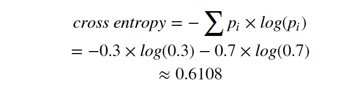
Most of us may have observed cases where deeper decision trees have lower cross entropy than shallower decision trees. For example, there are 30 black balls and 70 white balls in the bag,

Figure 1: root nodes with no extra layer
The cross entropy here is same as expected cross entropy:
Let’s add more features. Supposing these balls are made either in glass or in wood. For the 30 black balls, 20 of them are glass, 10 of them are wooden. For the 70 white balls, 41 of them are glass, 29 of them are wooden. We want to use this feature to help classify the color of balls, and add one more layer using this feature (glass or wood) for our decision tree.
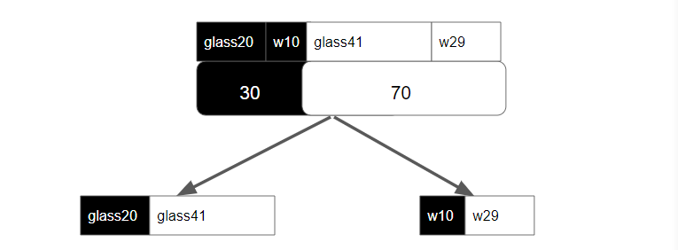
Figure 2: decision tree with more feature as extra layer for classification
Now the new expected cross entropy is:
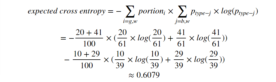
Here it is: 0.6079 < 0.6108. After adding one more layer, the expected cross entropy is lower than the original cross entropy. You can change the black/white numbers any way you like. However, I can not raise up any opposite examples which results in a higher expected cross entropy after adding more layers.
It draws my attention.
My intuition tells me this is a rule and there is something interesting behind it.
2. Let’s form our conjecture
Conjecture: the expected cross entropy will not increase after adding layers in the decision tree.
2.1 Intuition for the conjecture
Besides our observations, we have more intuitive believes supporting this conjecture.
Let’s first take a look at the cross entropy.

What does it mean? It is not only a bunch of logarithm calculations. Borrowing the ideas from physics (forget Shannon’s information theory for a while), entropy is a measurement for the degree of disorder or randomness. In our case, the definition of cross-entropy is like the one in physics, but more precisely, it is a measurement for the degree of purity on the leaf node.
A leaf node is more pure if the items it held is from a single type, than from mixed types. For example, leaf node (filled with cyan, each node holds only one item, of course it is pure) in figure 3.C is much purer than the root node in figure 3.A.
The expected cross-entropy, which is calculated as the weighted summation of cross-entropy on each leaf nodes, is a measurement of the linear combination for the degree of purity over all leaf nodes on the decision tree. For figure 3.C, the expected cross-entropy is 0 (linear combination of 0 is 0), lower than other cases (3.A, 3.B).
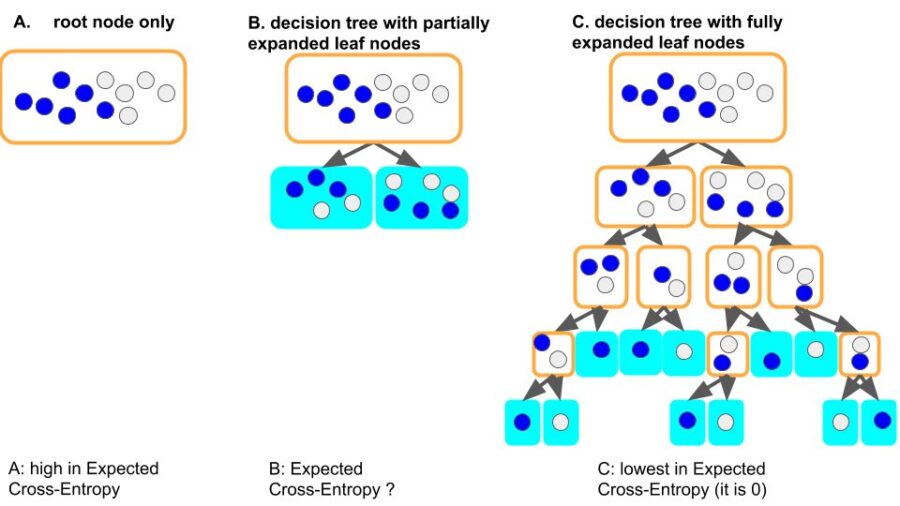
Figure 3: root node only (3.A), partially expanded tree (3.B), fully expanded tree (3.C). The leaf node in the fully expanded decision tree (figure 3.C, leaf nodes filled with cyan) is more pure than in the root node only scenario (figure 3.A).
Look at figure 3, our intuition tells us the following thing (ECE = expected cross-entropy):
ECE (3.A) >= ECE (3.B) >= ECE (3.C) = 0
This is consistent with our math conjecture, which can be written as:
- Inequality 1:
ECE (root node only) >= ECE (tree with 1 layer) >= ECE (tree with 2 layer) >= … >= ECE(fully expanded decision tree) = 0.
It will be beautiful if it is true. And we can prove it now.
3. Let’s prove it in Math
- Which part do we have to prove?
We are using a procedure like Mathematical Induction, but a little bit different. I know the Mathematical Induction should be applied as follows:
- prove 0 to 1, usually this part is the easiest part
- prove n to n+1, which is the hard part
What I would do, is:
- prove ECE(0 layer) >= ECE(1 layer), this part, however, is the most interesting part in the proof
- repetitively applying the result of 0 to 1, and prove the n to n+1. This part is relatively easier.
3.1. ECE(0 layer) >= ECE(1 layer)
First, let’s simplify the problem without lose of generality. We assume there are two types of balls in the bag, blue and gray. Each node will have two branches (left and right) if grow deeper.
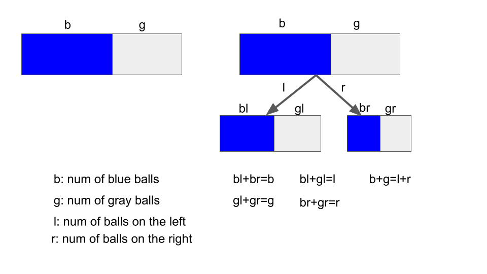
Figure 4. illustration of decision tree from 0 to 1.
According to figure 4, the inequality will be
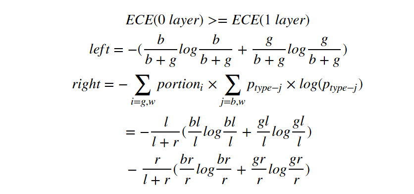
These items on the right hand can be written in another order:

From this formula, we will begin use the Jenson Inequality:
- Jenson Inequation: for concave function, f(E(x))>=E(f(x))
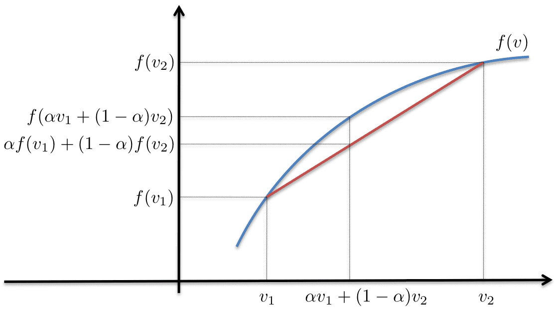
Figure 5. borrowed
We can write the Jenson inequality as:

Compare it with the right and left side of the inequality we want to prove:


We can prove the left >=right following:
- prove f(x) = – x * log(x) is concave. This is quite easy, using 2nd order derivative <=0.
- proving the following inequality.

I’ll only prove of the first line, and the second line is the same:
- from Jenson inequality (remember l+r = b+g)
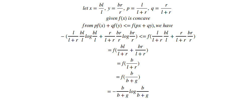
ECE(0 layer) >= ECE(1 layer) have done!
3.2. ECE(n layer) >= ECE(n+1 layer)
To prove ECE(n layer) >= ECE(n+1 layer), just use ECE(0 layer) >= ECE(1 layer) on each of the leaf node when further splitting the nth layer into n+1 layer.
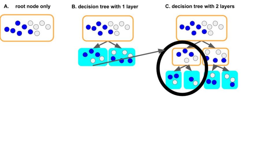
Figure 6. repetitively apply ‘0 to 1’ in proving ‘n to n+1’.
Then we have finished the proof. Our intuition didn’t lie!! It is true that deeper decision tree will never have higher expected cross-entropy than shallower decision tree.
4. Last word.
PS1. Jenson inequality is extremely powerful!
Jenson inequality is not difficult. I’ve been using it since middle school for Math Olympic Competition. But it is an MDW (Massive Destruction Weapon) in data science! We need use it in the theoretical speculation for decision tree, K-means, EM. It is very helpful!
PS2. Thanks to Entropy
Why are we able to implement Jenson inequality in the decision tree? It is because: 1. the cross-entropy function is concave, 2. expected cross-entropy is a linear combination of cross-entropy. These two factors are the keys to the ‘none-increasing entropy’ property for decision tree.
PS3. Is a lower expected cross-entropy what we really want in decision tree?
Sadly, the answer is NO. What we want from the classifier is its ability to distinguish different types of items. The ECE is an indirect index we use in decision tree. The lower expected cross-entropy only means the leaf nodes have higher degree of purity. It does not directly revealing the ability for the decision tree to recognize cat or dog. The lower ECE may be results from the fact that the decision tree is fully expanded and each of its node hold one item only. Surely it is pure, but it still stupid and it makes terrible guesses besides the existing samples. This is over-fitting.
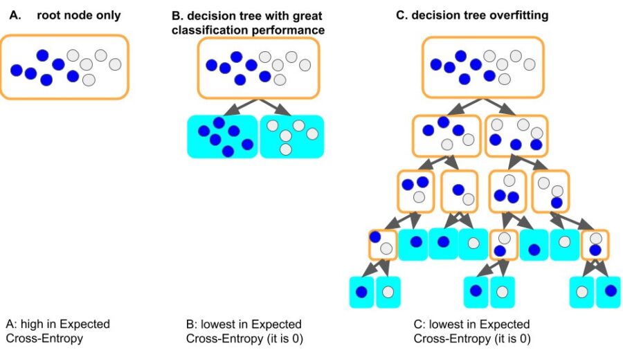
Figure 7. Lower Expected Cross-Entropy only means high degree of purity on the leaf nodes. It may lead to over-fitting.
From figure 7, you can clearly see the comparison between a good classifier (7.B) and an over-fitting tree (7.C), which are both lowest in Expected Cross-Entropy (=0). To avoid over-fitting, we need restrictions on the depth of the tree. What we want is a classifier like 7.B, not the pure but stupid 7.C.
Thanks for reading and I appreciate your feedbacks!