
In my earlier post I discussed how performing topological data analysis on the weights learned by convolutional neural nets (CNN’s) can give insight into what is being learned and how it is being learned.
The significance of this work can be summarized as follows:
- It allows us to gain understanding about how the neural network performs a classification task.
- It allows us to observe how the network learns
- It allows us to see how the various layers in a deep network differ in what they detect
In this post we show how one might leverage this kind of understanding for practical purposes. I will build on the work that Rickard Gabrielsson and I have done while discussing three other findings that we have discovered. Those are:
- How barcode lengths from persistent homology can be used to infer the accuracy of the CNN
- How our findings generalize from one dataset to the next
- How the qualitative nature of the datasets is quantitatively measurable using the persistent homology barcode approach
We need to recall some ideas from the previous post. One of the ideas introduced was the use of persistent homology as a tool for measuring the shape of data. In our example, we used persistent homology to measure the size and strength or “well-definedness” of a circular shape.
We’ll first recall the notions of persistent homology. Persistent homology assigns to any data set and dimension a “barcode”, which is a collection of intervals. In dimension = 0, the barcode output reflects the decomposition of the data set into clusters or components.
In clustering, one can choose a threshold and connect any two points by an edge if their distance is less than this threshold, and compute connected components of the resulting graph. Of course, as the threshold grows, more points will be connected, and we will obtain fewer clusters. The barcode is a way of tracking this behavior. The picture below gives an indication of how this works.
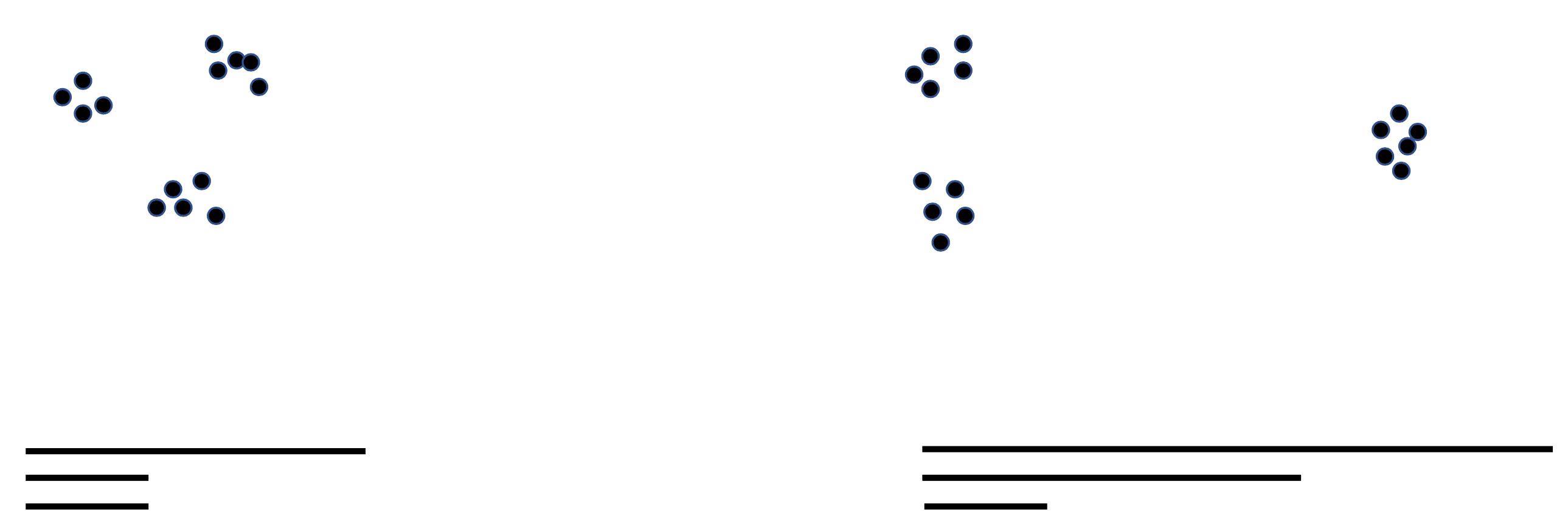
On the left, we have a data set that breaks naturally into three clusters, roughly equidistant. The barcode reflects that in the presence of three bars, with only one longer than a certain threshold value, depending on the distance between the clusters. The bars represent the initial clusters, with two of them cutting off at the threshold value where the clusters merge. On the right, we have a similar situation, except that the clusters are not equidistant. In this case, we begin with three bars because at a fine level of resolution, there are three clusters. At a threshold value roughly equal to the one on the left, we see that the two adjacent clusters merge into a single one, and we are looking at two clusters for a while. This is reflected in the barcode by the fact that the first bar is relatively short, while the other two are longer. Finally, as the threshold gets large enough to merge all three, we see that two of the bars are shorter than that threshold, with only one longer.

For higher dimensions, persistent homology measures the presence of geometric features beyond cluster decomposition. In the case of dimension = 1, the barcode measures the presence of loops in a data set.
On the left, the barcode consists of a long bar and some much shorter ones. The long bar reflects the presence of a circle whereas the shorter ones occur due to noise. On the right, we again have the short bars corresponding to noise and two longer bars, of different lengths. These bars reflect the presence of the two loops,and the different length of the bars correspond to the size of the loops. Length of a bar can also reflect what one might refer to as the “well-definedness” of the loop.
Let’s look at these images to understand that better.
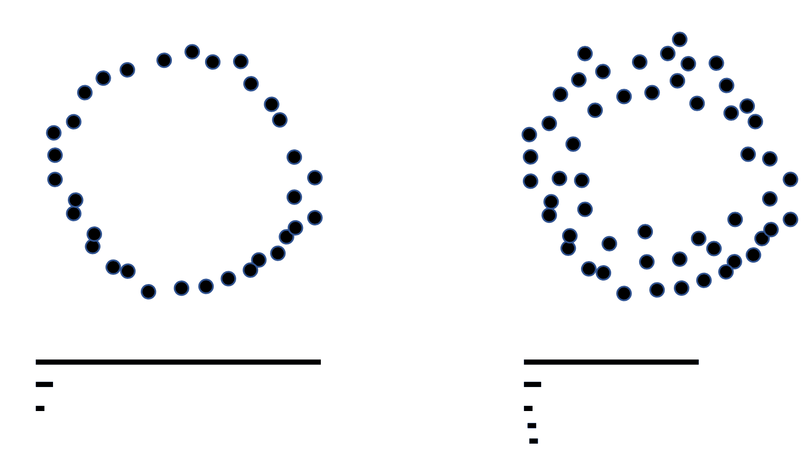
On the left we have a very well-defined loop, and its barcode. On the right, some noise has been added to the loop, making in more diffuse and less well-defined. The longest bar on the right is shorter than that on the left. The length of the longest bar can thus reflect the well-definedness of the loop.
Inferring the Accuracy of a CNN
In the earlier post, we saw that the “loopy” shapes obtained from Ayasdi’s software was in fact confirmed by the presence of a single long bar within the barcode. We now wanted to understand how the loopy shape evolved as the training progressed.
We achieved this by examining the correlation between the length of the longest bar in the barcode (which can be computed at any stage of training) and the accuracy at that point of training. We performed these computations for two data sets, MNIST and a second data set of house numbers, referred to as SVHN.
The results look like this:
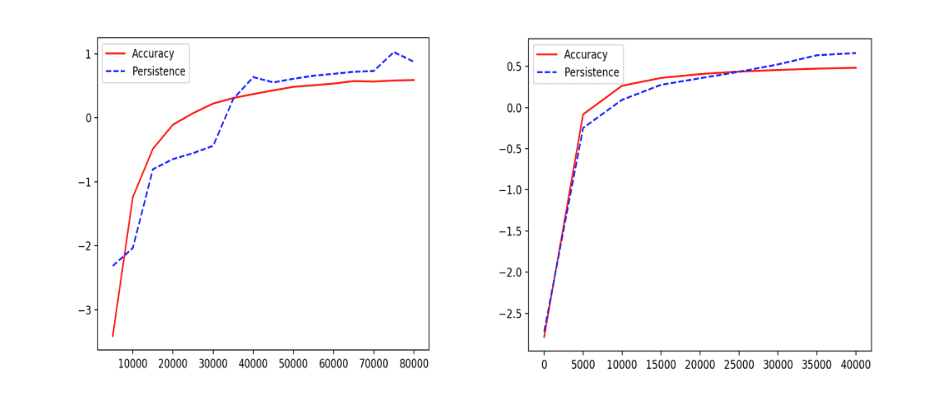
On the left is MNIST, on the right is SVHN. The x-axis records the number of iterations in the learning process. The y axis records the accuracy or length of longest bar in the barcode respectively, after mean centering and normalization.
As one can see, the length of the longest bar is well correlated with the accuracy of the classifier for the digits. This finding enhances the precision of our observations from the earlier post. There, we had only observed that, after training, we saw a single long bar in the barcode whereas we are now observing the length of the bar (and therefore the well-definedness of the circle) increasing as the training progresses.
Generalizing Across Data Sets
The second finding concerned the process of generalization from one dataset to another. Specifically, we trained a CNN based on MNIST, and examined its accuracy when applied to SVHN. We performed the training using three different methods.
- The standard procedure for a standard CNN
- Train the network by fixing the first convolutional layer to a random Gaussian
- Train the network by fixing the first convolutional layer to a perfect discretization of the primary circle found in MNIST
When we did this, we found that in the three separate cases, the accuracy of prediction on SVHN was 10% in case (1), 12% in case (2), and 22% in case (3). Of course, all these numbers are low accuracy numbers, but the results demonstrate that fixing the first convolutional layer to consist entirely of points from the primary circle model significantly improves the generalization from MNIST to SVHN. There are more complex models than the primary circle which one could include and expect to find further improvement in generalization.
Measuring Variability
The third finding involved an examination of the variability of the two datasets. Qualitatively we can determine that SVHN has much more variability than does MNIST. We would, in turn, expect that SVHN provides a richer data set and more precise data set of weight vectors. Indeed, persistence interval for SVHN is significantly longer than that for MINST (1.27 vs. 1.10). This further confirms from above, that there is a strong correlation between the “well-definedness” of the circle model generated and the quality of the neural network.
Summing Up
The reason topological analysis is useful in this type of analytical challenge is that it provides a way of compressing complicated data sets into understandable and potentially actionable form. Here, as in many other data analytic problems, it is crucial to obtain an understanding of the “frequently occurring motifs” within the data. The above observations suggest that topological analysis can be used to obtain control and understanding of the learning and generalization capabilities of CNN’s. There are many further ideas along these lines, which we will discuss in future posts.