This is the 2nd part of the article on a few applications of Fourier Series in solving differential equations. All the problems are taken from the edx Course: MITx – 18.03Fx: Differential Equations Fourier Series and Partial Differential Equations. The article will be posted in two parts (two separate blongs)

We shall see how to solve the following ODEs / PDEs using Fourier series:

Solve the PDE for Heat / Diffusion using Neumann / Dirichlet boundary conditions
Solve Wave equation (PDE).
Remove noise from an audio file with Fourier transform.

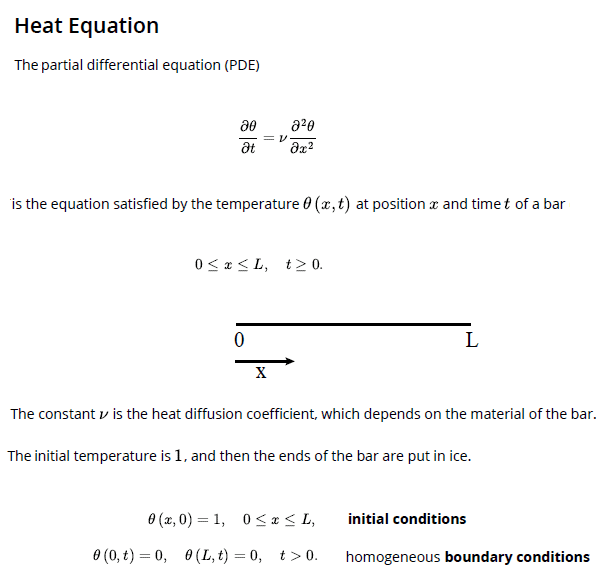
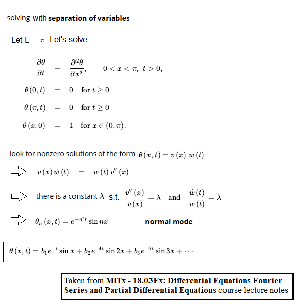
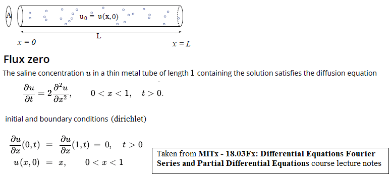
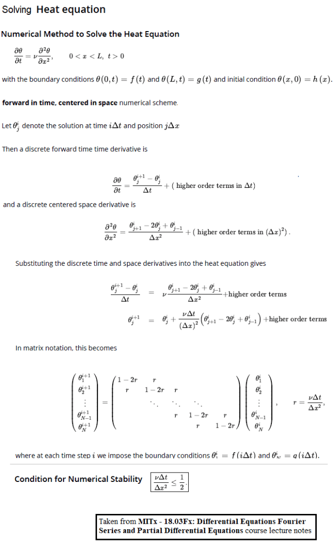
Heat / Diffusion Equation

The following animation shows how the temperature changes on the bar with time (considering only the first 100 terms for the Fourier series for the square wave).

Let’s solve the below diffusion PDE with the given Neumann BCs.

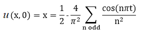
As can be seen from above, the initial condition can be represented as a 2-periodic triangle wave function (using even periodic extension), i.e.,

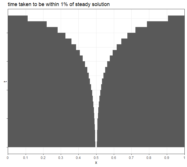
The next animation shows how the different points on the tube arrive at the steady-state solution over time.

The next figure shows the time taken for each point inside the tube, to approach within 1% the steady-state solution.

with the following

L=5, the length of the bar is 5 units.
Dirichlet BCs: u(0, t) =0, u(L,t) = sin(2πt/L), i.e., the left end of the bar is held at a constant temperature 0 degree (at ice bath) and the right end changes temperature in a sinusoidal manner.
IC: u(x,0) = 0, i.e., the entire bar has temperature 0 degree.

The following R code implements the numerical method:

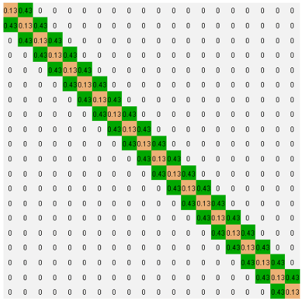
#Solve heat equation using forward time, centered space scheme
 
#Define simulation parameters
x = seq(0,5,5/19) #Spatial grid
dt = 0.06         #Time step
tMax = 20         #Simulation time
nu = 0.5          #Constant of proportionality
 
t = seq(0, tMax, dt) #Time vector
 
n = length(x)
m = length(t)
 
fLeft = function(t) 0                             #Left boundary condition
fRight = function(t) sin(2*pi*t/5)                #Right boundary condition
fInitial = function(x) matrix(rep(0,m*n), nrow=m) #Initial condition
 
#Run simulation
dx = x[2]-x[1]
r = nu*dt/dx^2
 
#Create tri-diagonal matrix A with entries 1-2r and r

The tri-diagonal matrix A is shown in the following figure

#Impose inital conditions
u = fInitial(x)
u[1,1] = fLeft(0)
u[1,n] = fRight(0)
 
for (i in 1:(length(t)-1)) {
 
   u[i+1,] = A%*%(u[i,])   # Find solution at next time step
   u[i+1,1] = fLeft(t[i])  # Impose left B.C.
   u[i+1,n] = fRight(t[i]) # Impose right B.C.
}

The following animation shows the solution obtained to the heat equation using the numerical method (in R) described above,

Wave Equation

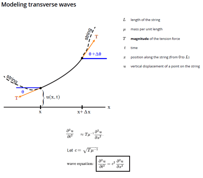
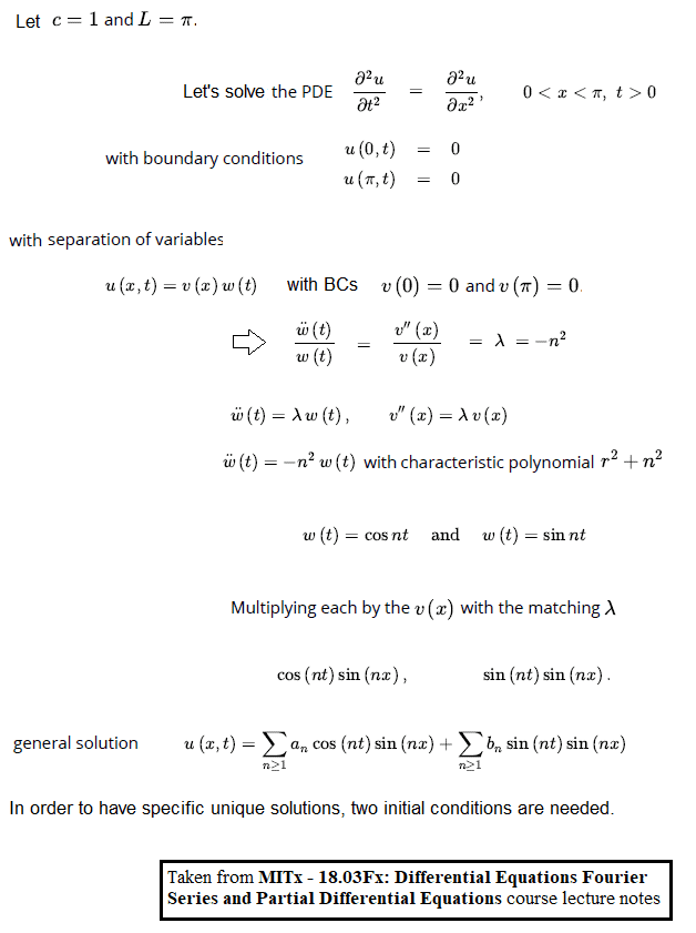
The next figure shows how can a numerical method be used to solve the wave PDE

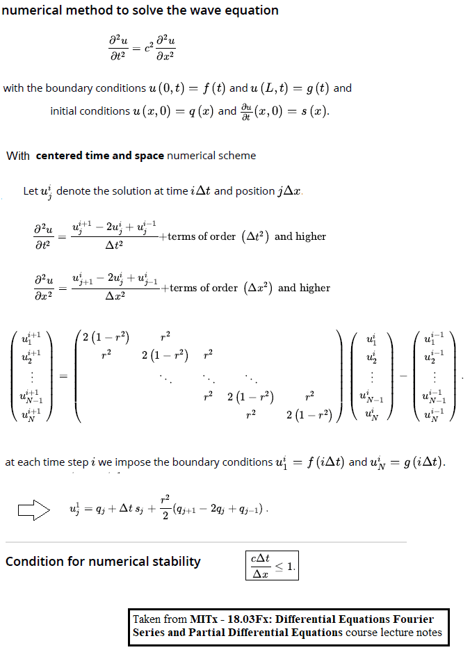
Implementation in R

#Define simulation parameters
x = seq(0,1,1/99) #Spatial grid
dt = 0.5 #Time step
tMax = 200 #Simulation time
c = 0.015 #Wave speed
 
fLeft = function(t) 0 #Left boundary condition
fRight = function(t) 0.1*sin(t/10) #Right boundary condition
fPosInitial = function(x) exp(-200*(x-0.5)^2) #Initial position
fVelInitial = function(x) 0*x #Initial velocity
 
#Run simulation
dx = x[2]-x[1]
r = c*dt/dx
 
n = length(x)
t = seq(0,tMax,dt)  #Time vector
m =length(t) + 1

Now iteratively compute u(x,t) by imposing the following boundary conditions

1. u(0,t) = 0
2. u(L,t) = (1/10).sin(t/10)

along with the following initial conditions

1. u(x,0) = exp(-500.(x-1/2)²)
2. ∂u(x,0)/∂t = 0.x

as defined in the above code snippet.

#Create tri-diagonal matrix A here, as described in the algorithm
 
#Impose initial condition
u = matrix(rep(0, n*m), nrow=m)
u[1,] = fPosInitial(x)
u[1,1] = fLeft(0)
u[1,n] = fRight(0)
 
for (i in 1:length(t)) {
 
  #Find solution at next time step
  if (i == 1) {
     u[2,] = 1/2*(A%*%u[1,]) + dt*fVelInitial(x)
  } else {
     u[i+1,] = (A%*%u[i,])-u[i-1,]
  }
 
  u[i+1,1] = fLeft(t[i]) #Impose left B.C.
  u[i+1,n] = fRight(t[i]) #Impose right B.C.
}

The following animation shows the output of the above implementation of the solution of wave PDE using R, it shows how the waves propagate, given a set of BCs and ICs.

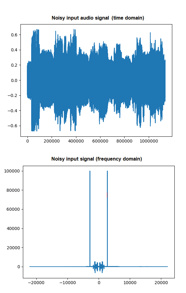
Some audio processing: De-noising an audio file with Fourier Transform

Let’s denoise an input noisy audio file (part of the theme music from Satyajit Ray’s famous movie পথের পাঁচালী, Songs of the road) using python scipy.fftpack module’s fft() implementation.

The noisy input file was generated and uploaded here.

from scipy.io import wavfile
import scipy.fftpack as fp
import numpy as np
import matplotlib.pylab as plt
 
# first fft to see the pattern then we can edit to see signal and inverse
# back to a better sound
Fs, y = wavfile.read('pather_panchali_noisy.wav') # can be found here: "https://github.com/sandipan/edx/blob/courses/pather_panchali_noisy.wav" data-mce-href="https://github.com/sandipan/edx/blob/courses/pather_panchali_noisy.wav".
 
# you may want to scale y, in this case, y was already scaled in between [-1,1]
Y = fp.fftshift(fp.fft(y))  #Take the Fourier series and take a symmetric shift
fshift = np.arange(-n//2, n//2)*(Fs/n)
 
plt.plot(fshift, Y.real) #plot(t, y); #plot the sound signal
plt.show()

You will obtain a figure like the following:

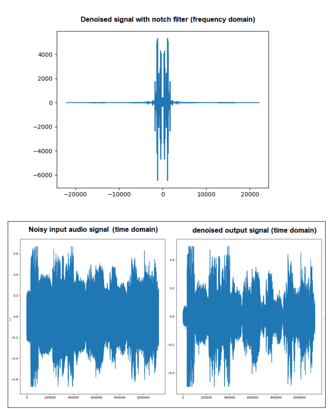
L = len(fshift) #Find the length of frequency values
Yfilt = Y
 
# find the frequencies corresponding to the noise here
print(np.argsort(Y.real)[::-1][:2])
# 495296 639296
 
Yfilt[495296] = Yfilt[639296] = 0  # find the frequencies corresponding to the spikes
plt.plot(fshift, Yfilt.real)
plt.show()
 
soundFiltered = fp.ifft(fp.ifftshift(Yfilt)).real
wavfile.write('pather_panchali_denoised.wav', Fs, soundNoisy)

The denoised output wave file produced with the filtering can be found here. (use vlc media player to listen to input and output wave files)

Fourier Series and Differential Equations with some applications in R and Python (Part 2)

Heat / Diffusion Equation

Wave Equation

Implementation in R

Some audio processing: De-noising an audio file with Fourier Transform