Feature Engineering with Tidyverse

In this blog post, I will discuss feature engineering using the Tidyverse collection of libraries. Feature engineering is crucial for a variety of reasons, and it requires some care to produce any useful outcome. In this post, I will consider a dataset that contains description of crimes in San Francisco between years 2003-2015. The data can be downloaded from Kaggle. One issue with this data is that there are only a few useful columns that are readily available for modelling. Therefore, it is important in this specific case to construct new features from the given data to improve the accuracy of predictions.

Among the given features in this data, the Address column (which is simply text) will be used to engineer new features. One can construct categorical variables from the Address column (there are a much smaller number of unique entries for addresses than the number of training examples) by one-hot encoding or by feature hashing. This is in principle possible, but creates around 20,000 new features. Given the size of the dataset, this makes training really slow. Instead, we can engineer features based on the crime counts in a given address . Looking through the kernels in Kaggle, I have come across an idea of creating ratios of crimes by Address. The idea is to construct numeric features using the ratio of each crime in a given category to the total crimes (of all categories) recorded in a given Address. Namely, I use the following as a numeric feature:

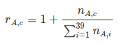
where n_(Ac) is the number of crimes of category c in a given address A. There are 39 different crime categories, which explains the limits of the sum in the denominator, while 1 is added to the ratio since I will compute the log of this feature eventually.

This idea is easy to implement (especially with Tidyverse functionalities), however requires some care. In a naive implementation, one would compute the crime by address ratios (defined above) for each Address in the training set. Then, these ratios can be merged with the testing set by the Address column. Doing so, one will immediately realize that this leads to overfitting. The reason is that we have used the target variable to construct the new features. As a result, the trained model found much higher weights for these features, since they are highly correlated to the target by construction. Thus, the model memorizes the data and cannot generalize properly when it encounters new data.

This looks pretty bad and it seems like constructing new features using the target is doomed. However, if one splits the training data into 2 pieces, and construct crime by address ratios from piece_1 and merge them with piece_2 (and repeat vice versa from piece_2 to piece_1) then the overfitting could be mitigated. The reason that this works is because the new features are constructed by using out-of-sample target values and so the crime by address ratios of each piece is not memorized.

As an illustration consider the following piece of example data:

Address	Category
A	ARSON
A	ARSON
A	BURGLARY
B	ARSON
C	ASSAULT
C	BURGLARY
E	ASSAULT
D	TRESPASS

Let’s split this data such that piece 1 contains rows (1,2,3,4,5,8) and piece 2 contains (6,7). Now, construct the crime by Address ratios (using the above formula) using piece 1, which would result in

Address	ARSON	ASSAULT	BURGLARY	TRESPASS
A	1.66	1.00	1.33	1.00
B	1.33	1.00	1.00	1.00
C	1.00	1.33	1.00	1.00
D	1.00	1.00	1.00	1.33

This is easily achieved by the spread function in tidyr library of Tidyverse. Now we can merge these with piece 2, which results in

Address	ARSON	ASSAULT	BURGLARY	TRESPASS
C	1	1.33	1	1
E	NA	NA	NA	NA

The NAs are the result of the fact that Address E was not a part of piece 1. In a large dataset, such NA values would reflect the fact that in that address there is not much crime, so one can impute them with the default value 1.0 (i.e. no crimes) as an approximation. This merge step is easily achieved by the left_join function of dplyr library of Tidyverse.

Now, it would be ideal to have more divisions of train so that each piece contains Address values that are present in the remaining pieces, so that a precise estimate of its crime by address feature can be constructed (thus fewer NAs would be encountered). This calls for the use of a k-folds division of train. This is in fact a reminiscent of the stacking predictions idea, which is used for combining predictions of different models, and to remove the bias on the best performing model.

Doing so, and engineering a few more (simpler) features from Address, I ended up with a large model matrix that we can train a model. By popular demand, the choice I made here is XGBoost. After training a tree booster (the details of which can be found in the link below), we end up with the following importance measures for each feature in our model matrix

In the above plot, one can see that the top three most important features are the log ratios of crimes per address in categories LARCENY_THEFT, OTHEROFFENSES and DRUG_NARCOTIC. Then comes hour (hour of day where crime has occurred/reported). The x-axis measures the gain, which is the improvement in multi-class log-loss brought by a feature to the branches it is on (read more details about feature importance here). This result shows that the engineered features have become the most important ones in the model!

Details of all the calculations and the code can be found in the following R Notebook. The code can also be downloaded from my Github repo.

This post was originally published on my personal site.

0 members like this