
This article describes a few approaches and algorithms for temporal neighborhood discretization from a couple of papers accepted and published in the conference ICDM (2009) and in the journal IDA (2014), authored by me and my fellow professors Dr. Aryya Gangopadhyay and Dr. Vandana Janeja at UMBC. Almost all of the texts / figures in this blog post are taken from the papers.
Neighborhood discovery is a precursor to knowledge discovery in complex and large datasets such as Temporal data, which is a sequence of data tuples measured at successive time instances. Hence instead of mining the entire data, we are interested in dividing the huge data into several smaller intervals of interest which we call as temporal neighborhoods. In this article we propose 4 novel of algorithms to generate temporal neighborhoods through unequal depth discretization:
- Similarity-based simple Merging (SMerg)
- Markov Stationary distribution based Merging (StMerg)
- Greedy Merging (GMerg)
- Optimal Merging with Dynamic Programming (OptMerg).
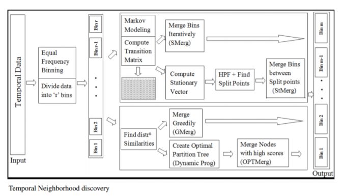
The next figure shows the schematic diagram of the four algorithms:
 https://sandipanweb.files.wordpress.com/2017/04/im03.png?w=150 150w, https://sandipanweb.files.wordpress.com/2017/04/im03.png?w=300 300w, https://sandipanweb.files.wordpress.com/2017/04/im03.png?w=768 768w, https://sandipanweb.files.wordpress.com/2017/04/im03.png 790w” sizes=”(max-width: 676px) 100vw, 676px” />
All the algorithms start by dividing a given time series data into a few (user-chosen) initial number of bins (with equal-frequency binning) and then they proceed merging similar bins (resulting a few possibly unequal-width bins) using different approaches, finally the algorithms terminate if we obtain the user-specified number of output (merged) bins .
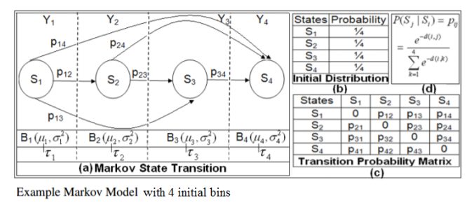
Both the algorithms SMerg and STMerg start by setting a Markov Model with the initial bins as the states (each state being summarized using the corresponding bin’s mean and variance) and Transition Matrix computed with the similarity (computed using a few different distribution-similarity computation metrics) in between the bins, as shown in the following figure:
 https://sandipanweb.files.wordpress.com/2017/04/im0_1.png?w=150 150w, https://sandipanweb.files.wordpress.com/2017/04/im0_1.png?w=300 300w, https://sandipanweb.files.wordpress.com/2017/04/im0_1.png 761w” sizes=”(max-width: 676px) 100vw, 676px” />
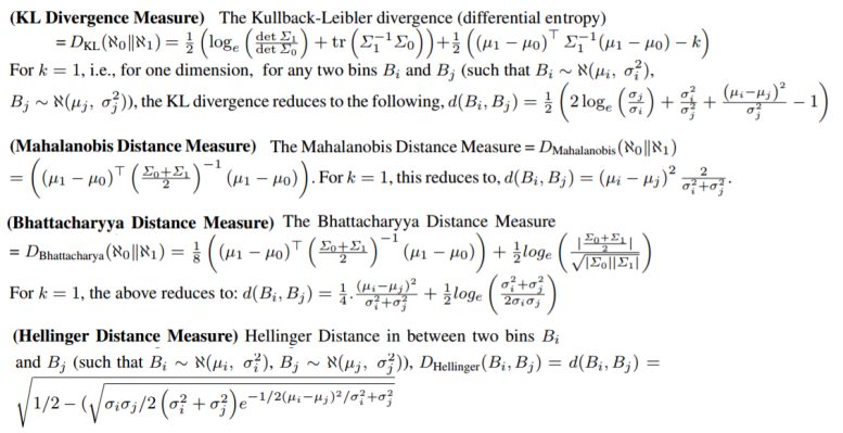
The following distribution-distance measures are used to compute the similarity in between the bins (we assume the temporal data in each of the bins as normally distributed with the bin mean and the variance).
 https://sandipanweb.files.wordpress.com/2017/04/im0_1_1.png?w=150&a… 150w, https://sandipanweb.files.wordpress.com/2017/04/im0_1_1.png?w=300&a… 300w, https://sandipanweb.files.wordpress.com/2017/04/im0_1_1.png?w=768&a… 768w, https://sandipanweb.files.wordpress.com/2017/04/im0_1_1.png?w=1024&… 1024w, https://sandipanweb.files.wordpress.com/2017/04/im0_1_1.png 1130w” sizes=”(max-width: 777px) 100vw, 777px” />
We discuss the results for a one dimensional special case here, however, our approach is generalizable to multidimensional temporal data.
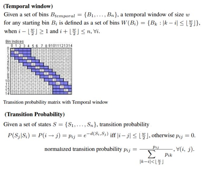
The Markov Transition Matrix is defined as shown in the following figure as a block-diagonal matrix with a given Temporal window size w.
 https://sandipanweb.files.wordpress.com/2017/04/im_0_1_21.png?w=150 150w, https://sandipanweb.files.wordpress.com/2017/04/im_0_1_21.png?w=300 300w, https://sandipanweb.files.wordpress.com/2017/04/im_0_1_21.png?w=768 768w, https://sandipanweb.files.wordpress.com/2017/04/im_0_1_21.png 823w” sizes=”(max-width: 676px) 100vw, 676px” />
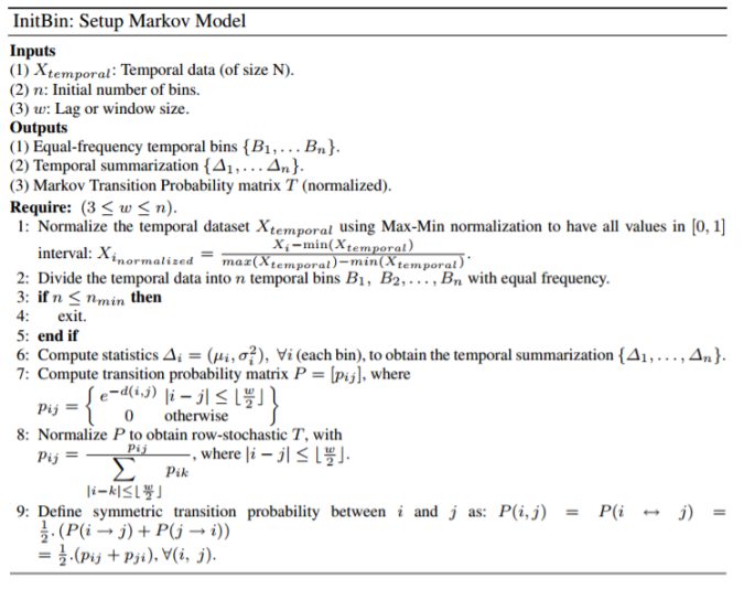
The following figure shows the pre-processing step Init-bin for setting up the Markov Model
 https://sandipanweb.files.wordpress.com/2017/04/im16.png?w=150 150w, https://sandipanweb.files.wordpress.com/2017/04/im16.png?w=300 300w, https://sandipanweb.files.wordpress.com/2017/04/im16.png 748w” sizes=”(max-width: 676px) 100vw, 676px” />
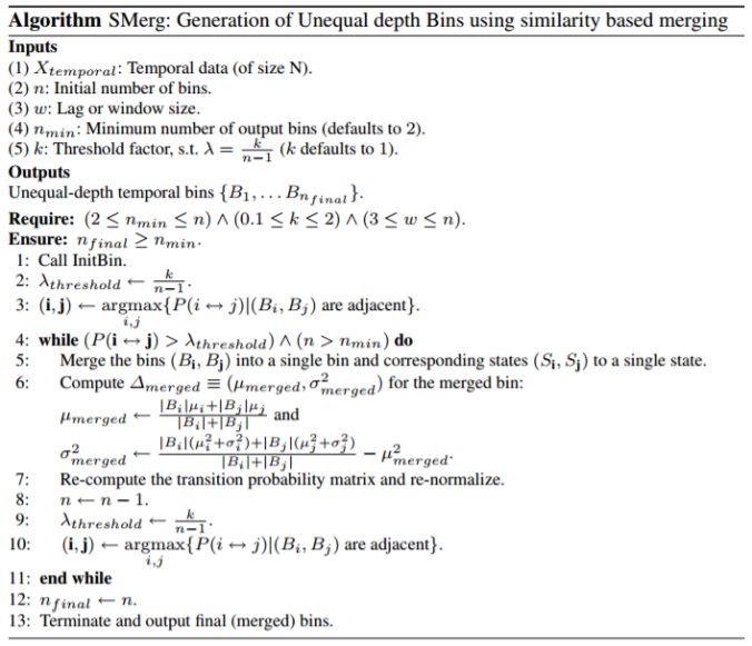
- Similarity based merging (SMerg)In this approach we iteratively merge highly similar bins (based on a threshold). At every iteration the transition matrix is recomputed since bin population has changed.
 https://sandipanweb.files.wordpress.com/2017/04/im23.png?w=150 150w, https://sandipanweb.files.wordpress.com/2017/04/im23.png?w=300 300w, https://sandipanweb.files.wordpress.com/2017/04/im23.png 707w” sizes=”(max-width: 676px) 100vw, 676px” />
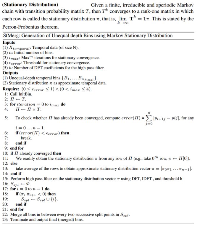
2. Markov Stationary distribution based Merging (StMerg)
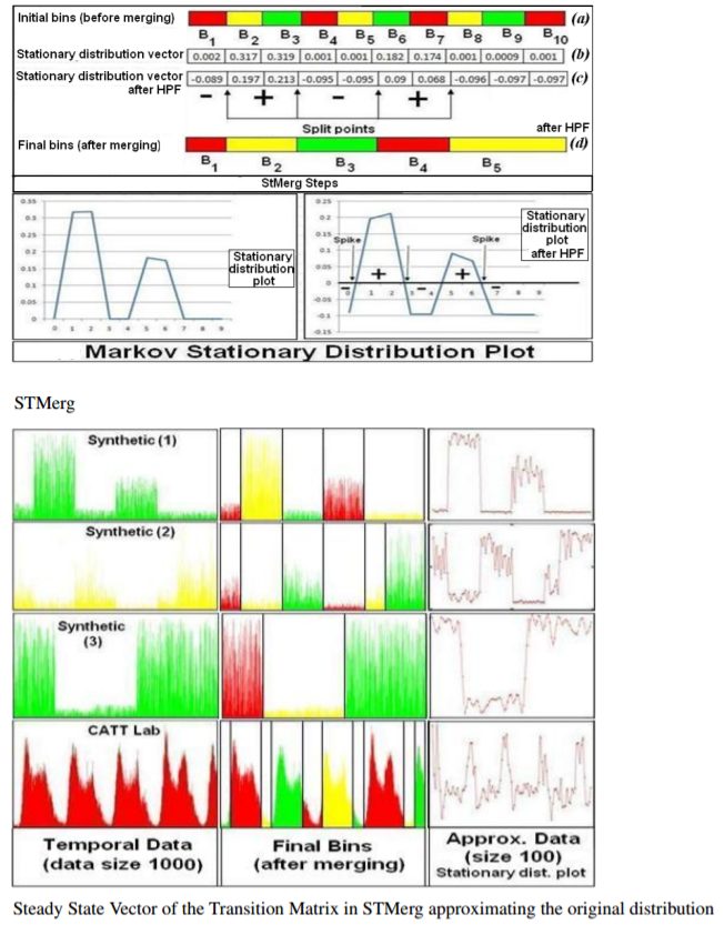
Given the initial equal-depth bins and the transition matrix T, we compute the steady-state vector at the stationary distribution, using power-iteration method. Once we have this vector we need to detect the spikes in the vector which indicate the split points such that the data on either side of any split point is very dissimilar and the data within two split points is highly similar. In order to detect these spikes we use Discrete Fourier Transform (DFT) and Inverse Discrete Fourier Transform (IDFT).
The following figure shows how the steady state vector approximate the pattern in the original data for a few synthetically generated and public transportation datasets, thereby achieving data compression (since number of states in the steady state vector =
# output bins obtained after bin merging # initial bins).
 https://sandipanweb.files.wordpress.com/2017/04/im44.png?w=116 116w, https://sandipanweb.files.wordpress.com/2017/04/im44.png?w=232 232w” sizes=”(max-width: 652px) 100vw, 652px” />
 https://sandipanweb.files.wordpress.com/2017/04/im33.png?w=132 132w, https://sandipanweb.files.wordpress.com/2017/04/im33.png?w=264 264w, https://sandipanweb.files.wordpress.com/2017/04/im33.png?w=768 768w, https://sandipanweb.files.wordpress.com/2017/04/im33.png 903w” sizes=”(max-width: 676px) 100vw, 676px” />
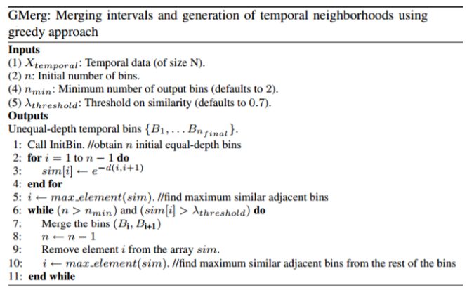
3. Greedy Approach (GMerg)
This algorithm starts with the initial bins and starts merging the most similar adjacent bins right away (does not require a Markov Model). It is greedy in the sense that it chooses the current most similar intervals for merging and hence may find a local optimum instead of obtaining a globally optimal merging.
 https://sandipanweb.files.wordpress.com/2017/04/im51.png?w=150 150w, https://sandipanweb.files.wordpress.com/2017/04/im51.png?w=300 300w, https://sandipanweb.files.wordpress.com/2017/04/im51.png 688w” sizes=”(max-width: 676px) 100vw, 676px” />
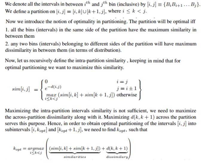
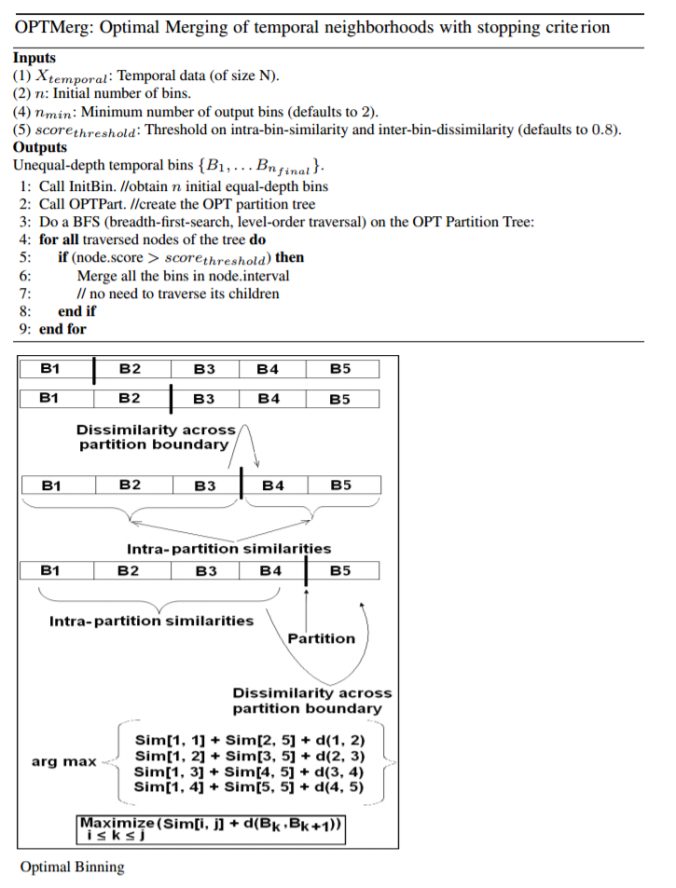
4. Optimal merging (OPTMerg)
Starting with the initial equal depth intervals (bins), we introduce the notion of optimal merging by defining optimal partitioning, as described in the following figures:
 https://sandipanweb.files.wordpress.com/2017/04/im5_6.png?w=150 150w, https://sandipanweb.files.wordpress.com/2017/04/im5_6.png?w=300 300w, https://sandipanweb.files.wordpress.com/2017/04/im5_6.png 761w” sizes=”(max-width: 676px) 100vw, 676px” />
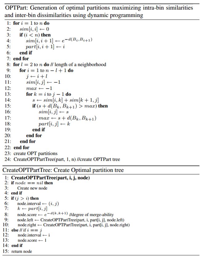
Next we use dynamic programming to find optimal partition, as shown in the next figure:
 https://sandipanweb.files.wordpress.com/2017/04/im61.png?w=120 120w, https://sandipanweb.files.wordpress.com/2017/04/im61.png?w=239 239w” sizes=”(max-width: 665px) 100vw, 665px” />
 https://sandipanweb.files.wordpress.com/2017/04/im7.png?w=114 114w, https://sandipanweb.files.wordpress.com/2017/04/im7.png?w=228 228w, https://sandipanweb.files.wordpress.com/2017/04/im7.png 725w” sizes=”(max-width: 676px) 100vw, 676px” />
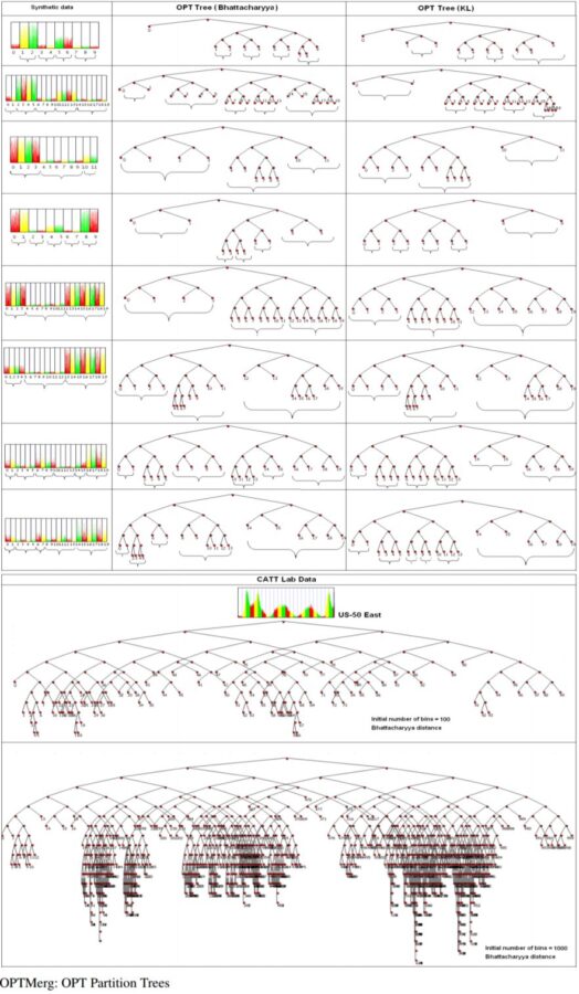
The following figures show the optimal partition trees obtained on a few datasets:
 https://sandipanweb.files.wordpress.com/2017/04/im8.png?w=120 120w, https://sandipanweb.files.wordpress.com/2017/04/im8.png?w=239 239w” sizes=”(max-width: 607px) 100vw, 607px” />
 https://sandipanweb.files.wordpress.com/2017/04/im9.png?w=87 87w, https://sandipanweb.files.wordpress.com/2017/04/im9.png?w=175 175w, https://sandipanweb.files.wordpress.com/2017/04/im9.png?w=768 768w, https://sandipanweb.files.wordpress.com/2017/04/im9.png?w=596 596w, https://sandipanweb.files.wordpress.com/2017/04/im9.png 1135w” sizes=”(max-width: 882px) 100vw, 882px” />
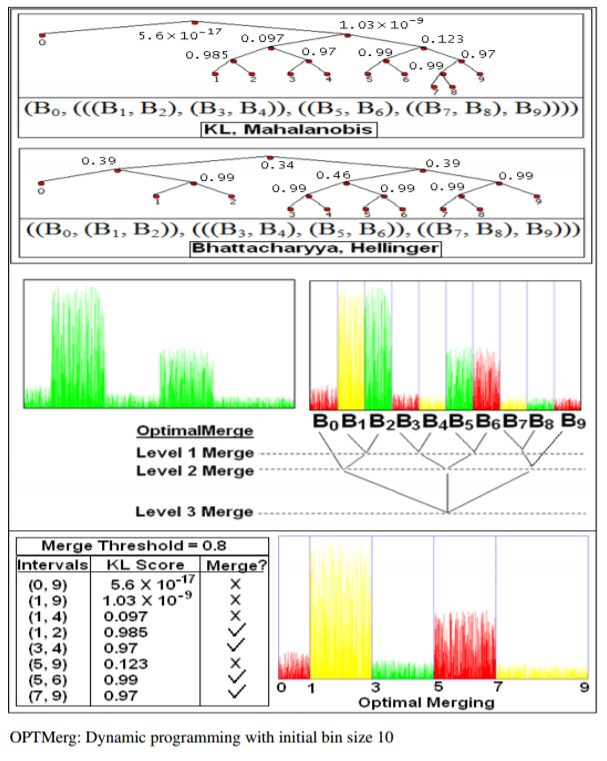
Experimental Results with Synthetic and CAT Lab data
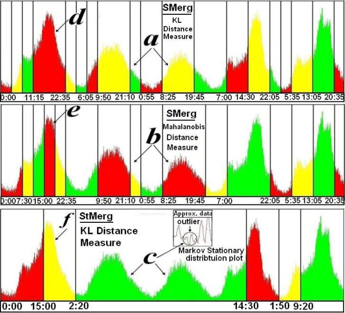
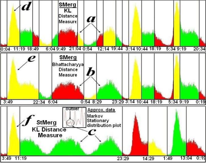
The following figures show the output bins obtained for few of the datasets using few of the algorithms and distance measures.
From the regions in the following figures marked (a, b) we can see that the weekend days are clearly different from the weekdays marked as (d, e). Further if we consider a very high level granularity such as the region (c) using StMerg with the KL distance we can entirely demarcate the weekends as compared to the weekdays (the global outliers can be detected, marked by a circle).
 https://sandipanweb.files.wordpress.com/2017/04/us-50-east.jpg?w=150 150w, https://sandipanweb.files.wordpress.com/2017/04/us-50-east.jpg?w=300 300w, https://sandipanweb.files.wordpress.com/2017/04/us-50-east.jpg 725w” sizes=”(max-width: 676px) 100vw, 676px” />
 https://sandipanweb.files.wordpress.com/2017/04/us-50-west.jpg?w=150 150w, https://sandipanweb.files.wordpress.com/2017/04/us-50-west.jpg?w=300 300w, https://sandipanweb.files.wordpress.com/2017/04/us-50-west.jpg 726w” sizes=”(max-width: 676px) 100vw, 676px” />
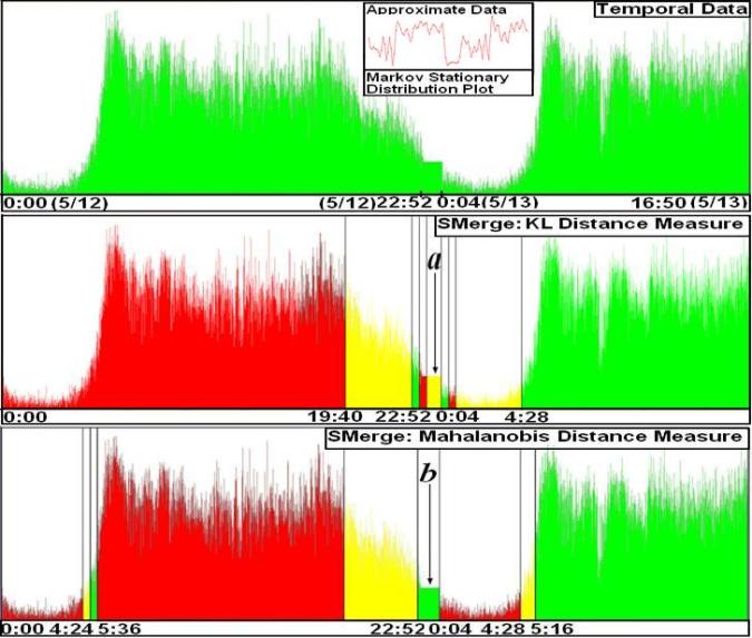
In the next figure, temporal interval (a) and (b) obtained after merging the intervals shows that there is an anomaly in the data from 05/12/2009 23 : 03 : 39 to 05/13/2009 00 03 39. We indeed find that speed value recorded by the censor is 20, constant all over the time period, and we verified from CATT lab representative that this is due to a possible ”free flow speed condition” where the sensor may go into a powersave mode if the traffic intensity is very minimal or close to zero.
 https://sandipanweb.files.wordpress.com/2017/04/i-395.jpg?w=150 150w, https://sandipanweb.files.wordpress.com/2017/04/i-395.jpg?w=300 300w, https://sandipanweb.files.wordpress.com/2017/04/i-395.jpg 727w” sizes=”(max-width: 676px) 100vw, 676px” />
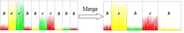
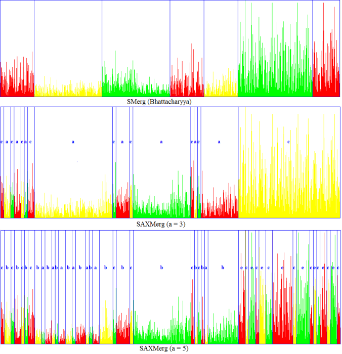
We also have extended the existing well-known and popular technique SAX (Symbolic Aggregate Approximation) to SAXMerg (where we merge the adjacent bins represented by same symbol) as shown below.
 https://sandipanweb.files.wordpress.com/2017/04/sax.png?w=150 150w, https://sandipanweb.files.wordpress.com/2017/04/sax.png?w=300 300w” sizes=”(max-width: 646px) 100vw, 646px” />
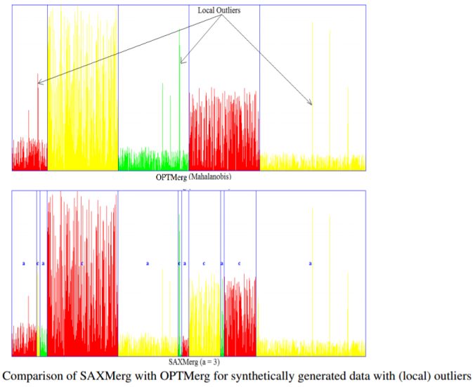
We then compare our results with those obtained using SAXMerg, as shown in the following figures.
It can be seen from the merged output bins from the next figure, the OPTMerg with Mahalanobis distance measure is more robust to local outliers than the SAXMerg is.
 https://sandipanweb.files.wordpress.com/2017/04/im10.png?w=150 150w, https://sandipanweb.files.wordpress.com/2017/04/im10.png?w=300 300w, https://sandipanweb.files.wordpress.com/2017/04/im10.png?w=768 768w, https://sandipanweb.files.wordpress.com/2017/04/im10.png 886w” sizes=”(max-width: 676px) 100vw, 676px” />
 https://sandipanweb.files.wordpress.com/2017/04/saxcomp.png?w=145 145w, https://sandipanweb.files.wordpress.com/2017/04/saxcomp.png?w=290 290w, https://sandipanweb.files.wordpress.com/2017/04/saxcomp.png?w=768 768w, https://sandipanweb.files.wordpress.com/2017/04/saxcomp.png 1007w” sizes=”(max-width: 676px) 100vw, 676px” />
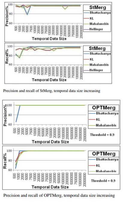
Some results with precision and recall:
 https://sandipanweb.files.wordpress.com/2017/04/im111.png?w=96 96w, https://sandipanweb.files.wordpress.com/2017/04/im111.png?w=191 191w” sizes=”(max-width: 430px) 100vw, 430px” />