
Till your good is better and better is best!
ENSEMBLE
Yes, the above quote is so true. We humans have ability to rate things and find some or the other matrices to measure things and evaluate them or their performances. Similarly, in Data Science you can measure your model’s accuracy and performance! The very first model that you build, you can set its matrices from the results and these matrices become your benchmark. Moving ahead you strive to or try to make other models on the same data which can break those benchmark. Which can predict better, which has better accuracy and so on… matrices can be anything. This vital technique is known as ‘Ensemble’ where you build one model, set its performance as measuring matrices and try to build other models which are better performers then previous matrices. This is the topic of the week! We will learn how to Ensemble models on a very interesting “Diabetes” data.
THE DATA
This data is taken from Kaggle and its best description is as follows provided on the portal: “The data was collected and made available by “National Institute of Diabetes and Digestive and Kidney Diseases” as part of the Pima Indians Diabetes Database. Several constraints were placed on the selection of these instances from a larger database. In particular, all patients here belong to the Pima Indian heritage (subgroup of Native Americans), and are females of ages 21 and above. ” Below is the R-Console Summary and Structure of this Data for better interpretation:
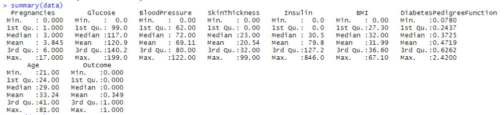
Summary of Diabetes Data
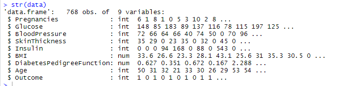
Structure of Diabetes Data
Here, for this data we will build models to predict the “Outcome” i.e. Diabetes Yes or No and we will perform Ensemble techniques to better our predictions. We will be using several techniques to do that, each technique is briefed as we keep building our codes below. Here is the link to this data from where it can be downloaded.
https://www.kaggle.com/kandij/diabetes-dataset
THE MODEL
EDA – Exploratory Data Analysis
This is typically done to better understand our data before we actually start building our models. This model has a lot to do with CARET library of R. CARET has few functions from which you can easily plot some graphs for EDA – Exploratory Data Analysis. Below is the listings for loading the data and computing some EDA plots.
Scatter plot Matrix
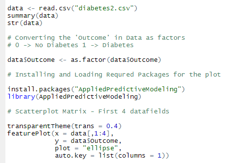
Listing for Loading Data and First 4 data field Scatter plot
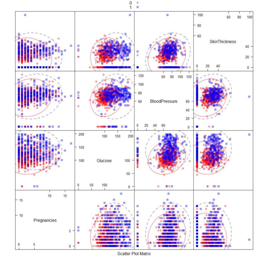
Scatter plot matrix for first 4 Diabetes Data fields
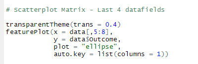
Listing for Scatter plot matrix of last 4 data fields
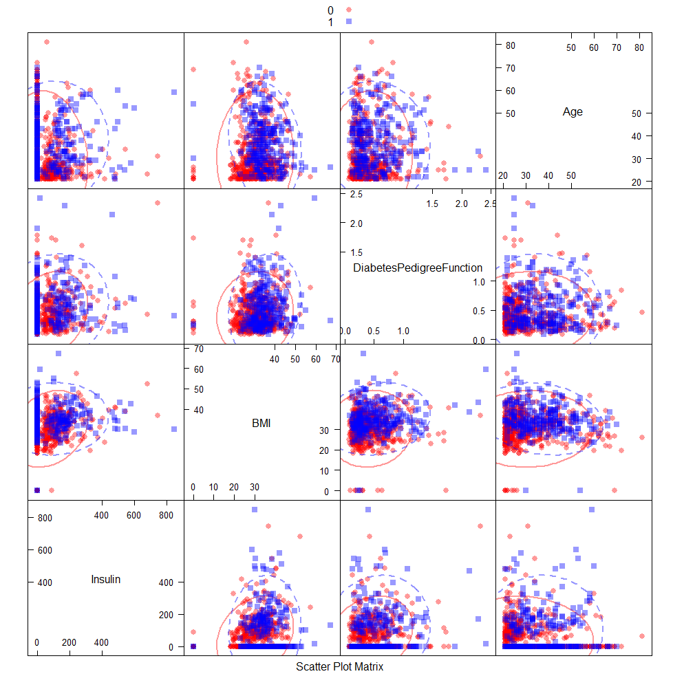
Scatter plot matrix for last 4 Diabetes Data fields
Overlayed Density plots
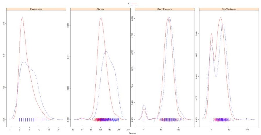
Overlayed Density plots of first 4 data fields
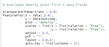
Listing for Overlayed Density plot for last 4 data fields
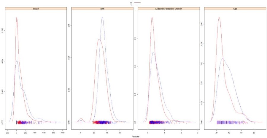
Overlayed Density plots of last 4 data fields
Box Plots
Listing for Box plot of first 4 data fields
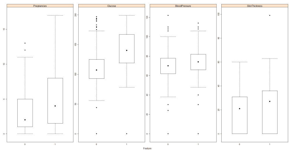
Box plots for first 4 data fields
Listings for Box Plot of last 4 data fields
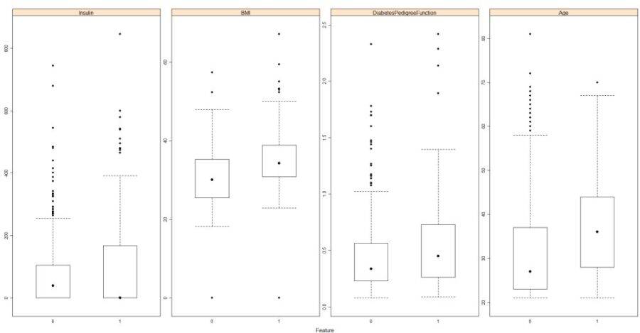
Box plots for last 4 data fields
Just eyeballing through and juggling around all the plots above you can get a better idea of the data. This is why we do EDA to better understand our data.
KNN – Model
The very first model we will be building is ‘k nearest neighbor’ model. Further, for this model we will be using 10 folds cross validation and 10 repeats to evaluate the model performance and for the output we will focus on the accuracy. The accuracy for this model will be our benchmark for Ensemble. Below are the listings for building the knn model.
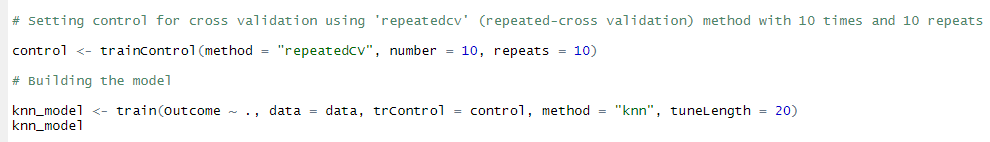
Listing for building knn model
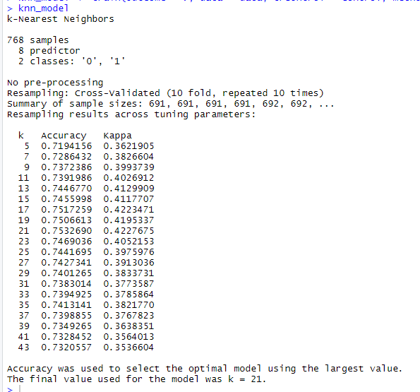
knn model output
As we can see above with 10 folds cross validation and 10 times repetition the best model formed was for k = 21 and equivalent accuracy for k = 21 is 0.7532 or 75.32%. This value is our bench mark value. Moving ahead building ensemble models we will strive to attain an accuracy better then 75.32%.
Bagging
Bagging or Bootstrapping Aggregation is a process in which for any given data set multiple random subsets of data set is created. By running an algorithm on these data sets it is possible that same data samples get picked up in multiple subsets.Below is the listing for building bagging model and we will be building “tree bag” method for bagging.
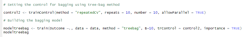
Listing for building bagging model
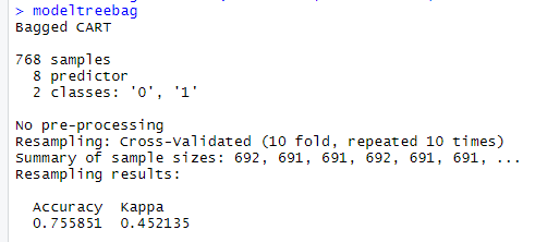
Output of Bagging model
The above is the output of the bagging model, and here there is a small hike in the model accuracy from 75.32% we have attained an accuracy of 75.58%. This is not a big leap but still a better version of the model in terms of accuracy.
Random Forests Model
Our next model is the Random forests model. They consists of a large number of individual decision trees and each tree splits out in class prediction and the class. With the majority rule and class with most votes is the output. Below is the listing for building Random forests model.
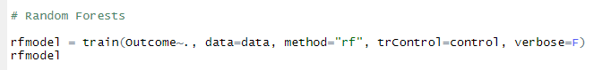
Listing for building random forests model
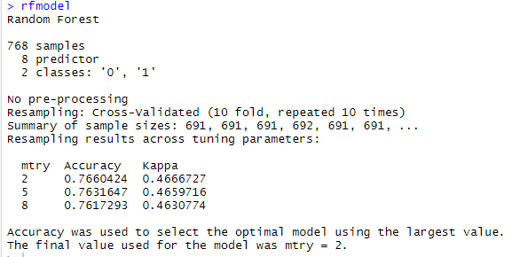
Random forests model
As we see above random forests model gives the accuracy for mtry = 2 which is 76.60% which is again better then our knn model accuracy of 75.32%.
Boosting
This is how boosting works, it builds the model with the with a Machine Learning algorithm that does predictions on entire data set.In these predictions there are some misclassified instances that are used for the second model. The second model learns from the misclassified instances of the first model. This process is goes on until the stopping process. The final output is voted from all the outcomes. There are number of Boosting algorithms we will be working with Gradient Boosting Machines (GBM) and XGBoost.
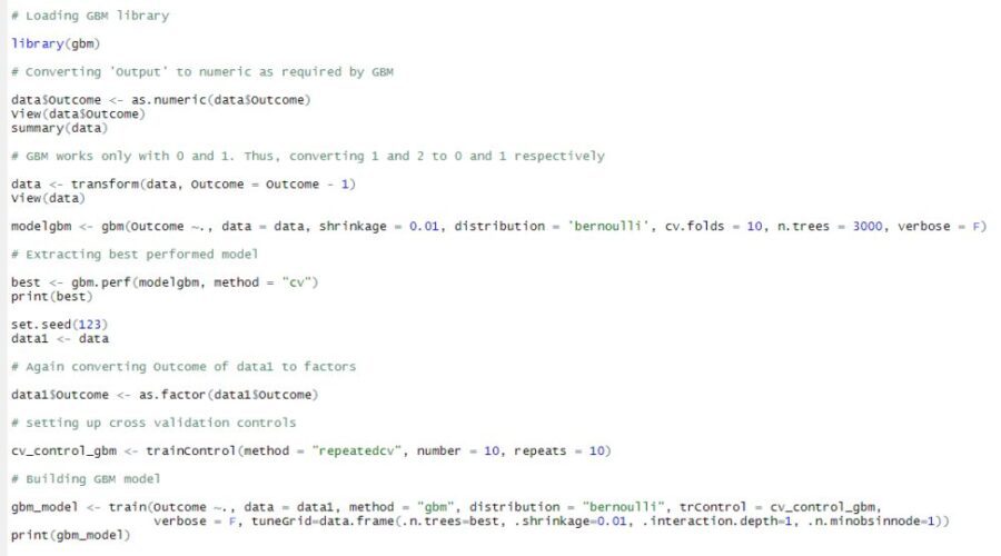
Listing for building GBM Model
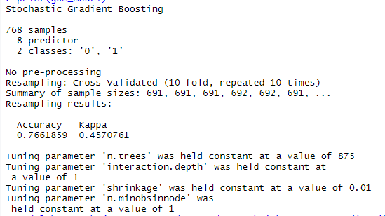
Output of Boosting Model
With the boosting model we got the accuracy of 76.61% again a better accuracy then knn which was 75.32%.
XGBoost
Below is the listing for XGBoost
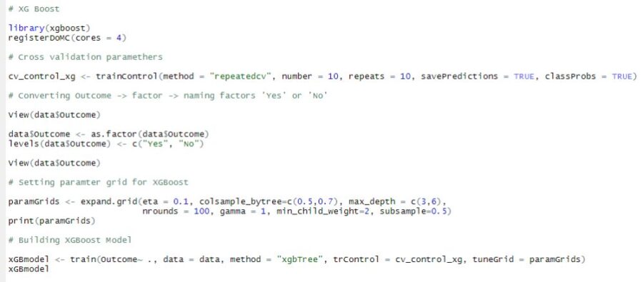
Listing for XGBoost
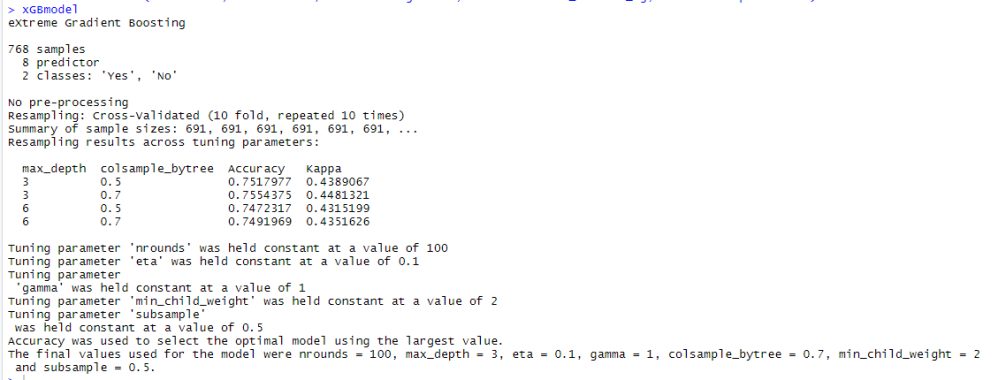
Output of XGBoost
The above output states that the best model is one with colsample_bytree = 0.7 and max_depth = 3 was selected. And for that model the accuracy is 75.54% again which is better then our knn model accuracy.
Stacking
This is very interesting model to end with. Can be called as model of models that too without manipulations. And what does that mean? So far, we have built the models which were exposed to subset of data and not actual entire data and its relationship. Stacking runs multiple Machine Learning Algorithms (the ones we mention) on the entire original data set. Stacking gets the combined power of several ML algorithms through getting the final prediction by means of voting or averaging as we do in other types of ensembles. Below is the listing for building stacking model.
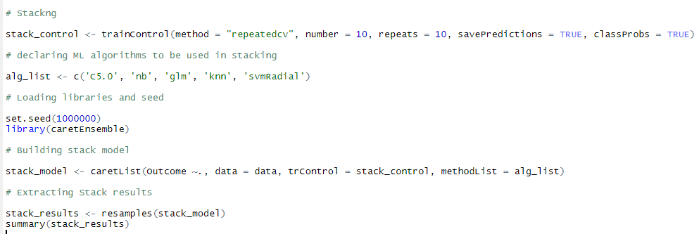
Listing for Stacking
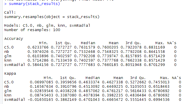
Stacking results
Stacking gives us a plethora of output from which we can analyze the best outcome from multiple ML algorithms. In the results above if we look for accuracy, mean and median all the accuracy are above our knn-accuracy of 75.32. The highest accuracy that could be attained across all the models is 87.01% which is way better than our knn accuracy.
CONCLUSION
- Ensemble models can be deployed to get better results thus enhancing our final model performance
- The highest accuracy that we could attain is 87.01% which is much higher than our accuracy of first knn-model accuracy of 75.32%
- To go beyond ensemble one can focus on Feature engineering of the model
This is all about ensemble modeling in data science, where we keep pushing the boundaries of our model matrices so that we can improve our model performance hence increase or model impact on the data-driven decision. It will always be a wise idea to use these techniques to better our model results rather than just building a single model and deploying it.
Read more here.