Data Science Simplified Part 7: Log-Log Regression Models

In the last few blog posts of this series, we discussed simple linear regression model. We discussed multivariate regression model and methods for selecting the right model.

Fernando has now created a better model.

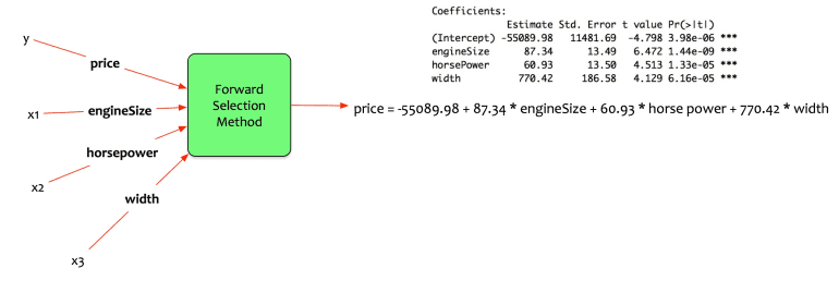
price = -55089.98 + 87.34 engineSize + 60.93 horse power + 770.42 width

Fernando contemplates the following:

How can I estimate the price changes using a common unit of comparison?
How elastic is the price with respect to engine size, horse power, and width?

In this article will address that question. This article will elaborate about Log-Log regression models.

The Concept:

To explain the concept of the log-log regression model, we need to take two steps back. First let us understand the concept of derivatives, logarithms, exponential. Then we need understand the concept of elasticity.

Derivatives:

Let us go back to high school math. Meet derivatives. One of most fascinating concepts taught in high school math and physics.

Derivate is a way to represent change – the amount by which a function is changing at one given point.

A variable y is a function of x. Define y as:

y = f(x)

We apply derivative on y with respect to x and represent it as follows:

dy/dx = df(x)/dx = f’(x)

This means the following:

The change in y with respect to change in x i.e. How much will y change if x changes?

Isn’t it that Fernando wants? He wants to know the change in price (y) with respect to changes in other variables (cityMpg and highwayMpg).

Recall that the general form of a multivariate regression model is the following:

y = β0 + β1.x1 + β2.x2 + .... + βn.xn + ε

Let us say that Fernando builds the following model:

price = β0 + β1 . engine size i.e. expressing price as a function of engine size.

Fernando takes the derivative of price with respect to engine size. Shouldn’t he be able to express the change in price with respect to changes in engine size?

Alas, it is not that simple. The linear regression model assumes a linear relationship. The Linear relationship is defined as:

y = mx + c

If the derivative of y over x is computed, it gives the following:

dy/dx = m . dx/dx + dc/dx

The change of something with respect to itself is always 1 i.e. dx/dx = 1
The change of a constant with respect to anything is always 0. That is why it is a constant. It won’t change. i.e. dc/dx = 0

The equation now becomes:

dy/dx = m

Applying derivate to price on engine size will yield nothing but the coefficient of engine size.

There has to be a way to transform it. Here come two more mathematical characters. Meet exponential and logarithms.

Exponentials:

Now let us look at exponential. This character is again a common character in high school math. An exponential is a function that has two operators. A base (b) and an exponent (n). It is defined as bn. it takes the form:

f(x) = bx

The base can be any positive number. Again Euler’s number (e) is a common base used in statistics.

Geometrically, an exponential relationship has following structure:

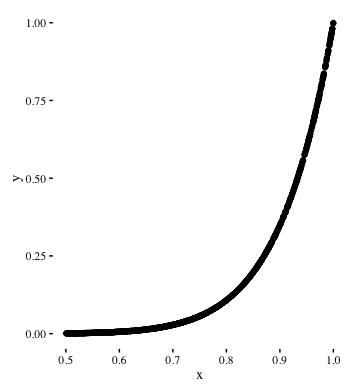
An increase in x doesn’t yield a corresponding increase in y. Until a threshold is reached.
After the threshold, the value of y shoots up rapidly for a small increase in x.

Logarithms:

The logarithm is an interesting character. Let us only understand its personality applicable for regression models. The fundamental property of a logarithm is its base. The typical base of the logarithm is 2, 10 or e.

Let us take an example:

How many 2s do we multiply to get 8? 2 x 2 x 2 = 8 i.e. 3
This can also be expressed as: log2(8) = 3

The logarithm of 8 with base 2 is 3

There is another common base for logarithms. It is called as “Euler’s number (e).” Its approximate value is 2.71828. It is widely used in statistics. The logarithm with base e is called as Natural Logarithm.

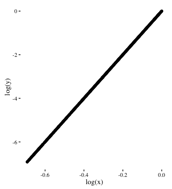
It also has interesting transformative capabilities. It transforms an exponential relation into a linear relation. Let us look at an example:

The diagram below, shows an exponential relationship between y and x:

If logarithms are applied to both x and y, the relationship between log(x) and log(y) is linear. It looks something like this:

Elasticity:

Elasticity is the measurement of how responsive an economic variable is to a change in another.

Say that we have a function: Q = f(P) then the elasticity of Q is defined as:

E = P/Q x dQ/dP

dq/dP is the average change of Q wrt change in P.

Bringing it all together:

Now let us bring these three mathematical characters together. Derivatives, Logarithms and Exponential. Their rules of engagement are as follows:

Logarithm of e is 1 i.e. log(e) = 1
The logarithm of an exponential is exponent multiplied by the base.
Derivative of log(x) is : 1/x

Let us take an example. Imagine a function y expressed as follows:

y = b^x.
=> log(y) = x log (b)

So does it mean for linear regression models? Can we do mathematical juggling to make use of derivatives, logarithms, and exponents? Can we rewrite the linear model equation to find the rate of change of y wrt change in x?

First, let us define relationship between y and x as an exponential relationship

y = α x^β
Let us first express this as a function of log-log: log(y) = log(α) + β.log(x)
Doesn’t equation #1 look similar to regression model: Y= β0 + β1 . x1 ? where β0 = log(α); β1 = β. This equation can be now rewritten as: log(y) = β0 + β1. log(x1)
But how does it represent elasticity? Let us take derivative of log(y) wrt x, we get the following:

d. log(y)/ dx = β1. log(x1)/dx.=> 1/y . dy/dx = β1 . 1/x => β1 = x/y . dy/dx.
The equation of β1 is the elasticity.

Model Building:

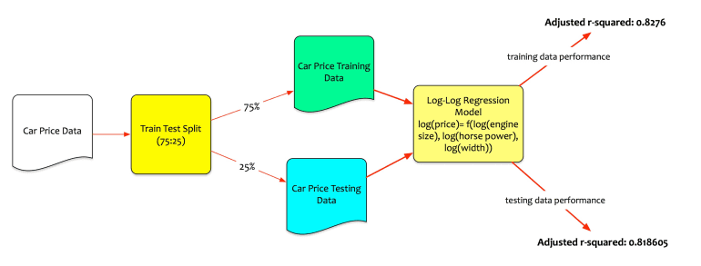
Now that we understand the concept, let us see how Fernando build a model. He builds the following model:

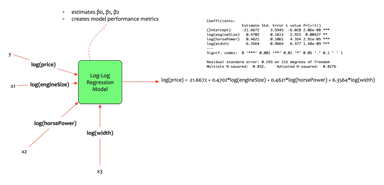
log(price) = β0 + β1. log(engine size) + β2. log(horse power) + β3. log(width)

He wants to estimate the change in car price as a function of the change in engine size, horse power, and width.

Fernando trains the model in his statistical package and gets the following coefficients.

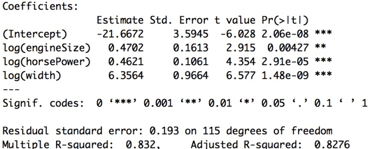
The equation of the model is:

log(price) = -21.6672 + 0.4702.log(engineSize) + 0.4621.log(horsePower) + 6.3564 .log(width)

Following is the interpretation of the model:

All coefficients are significant.
Adjusted r-squared is 0.8276 => the model explains 82.76% of variation in data.
If the engine size increases by 4.7% then the price of the car increases by 10%.
If the horse power increases by 4.62% then the price of the car increases by 10%.
If the width of the car increases by 6% then the price of the car increases by 1 %.

Model Evaluation:

Fernando has now built the log-log regression model. He evaluates the performance of the model on both training and test data.

Recall, that he had split the data into the training and the testing set. The training data is used to create the model. The testing data is the unseen data. Performance on testing data is the real test.

On the training data, the model performs quite well. The adjusted R-squared is 0.8276 => the model can explain 82.76% variation on training data. For the model to be acceptable, it also needs to perform well on testing data.

Fernando tests the model performance on test data set. The model computes the adjusted r-squared as 0.8186on testing data. This is good. It means that model can explain 81.86% of variation even on unseen data.

Note that the model estimates the log(price) and not the price of the car. To convert the estimated log(price) into the price, there needs to be a transformation.

The transformation is treating the log(price) as an exponent to the base e.

e^log(price) = price

Conclusion:

The last few posts have been quite a journey. Statistical learning laid the foundations. Hypothesis testing discussed the concept of NULL and alternate hypothesis. Simple linear regression models made regression simple. We then progressed into the world of multivariate regression models. Then discussed model selection methods. In this post, we discussed the log-log regression models.
So far the regression models built had only numeric independent variables. The next post we will deal with concepts of interactions and qualitative variables.