
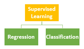
In the last blog post of this series, we discussed classifiers. The categories of classifiers and how they are evaluated were discussed. We have also discussed regression models in depth. In this post, we dwell a little deeper in how regression models can be used for classification tasks.
Logistic Regression is a widely used regression model used for classification tasks. As usual, we will discuss by example. No Money bank approaches us with a problem. The bank wants to build a model that predicts which of their customers will default on their loans. The dataset provided is as follows:

The features that will help us to build the model are:
- Customer Id: A unique customer identification
- Credit Score: A value between 0 and 800 indicating the riskiness of the borrower’s credit history.
- Loan Amount: This is the loan amount that was either completely paid off or the amount that was defaulted.
- Years in current job: A categorical variable indicating how many years the customer has been in their current job.
- Years of Credit History: The years since the first entry in the customer’s credit history
- Monthly Debt: The customer’s monthly payment for their existing loans
- The number of Credit Problems: The number of credit problems in the customer records.
- IsDefault: This is the target. If the customer has defaulted then it will 1 else it 0.
This is a classification problem.
Logistic regression is an avatar of the regression model. It transforms the regression model to become a classifier. Let us first understand why a vanilla regression model doesn’t work as a classifier.
The target is default has a value of 0 or 1. We can reframe this as a probability. The reframing is as follows:
- if probability of default >= 0.5 then the customer will default i.e. IsDefault = 1
- if probability of default < 0.5 then the customer will not default i.e. IsDefault = 0
Recall our discussion on Linear Regression Model. In the regression model, we had defined an dependent variable y which was a function of independent variables. For sake of simplicity, let us assume that we have only one independent variable x. The equation becomes:
y = β0 + β1 x
- β0 is the intercept.
- β1 is the coefficient of x.
In the example of loan default model, Tim uses credit score as the independent variable. The dependent variable (y) is the estimate of the probability that the customer will default i.e. P(default).
The equation can be written as:
P(default) = β0 + β1.credit score
Tim runs the regression model on the statistical package. The statistical package provides the following coefficient for β0 and β1:
- β0 = 0.73257
- β1 = -9.9238e-05
The equation to estimate the probability of default now becomes:
P(default) = 0.73257 + -9.9238e-05 . credit score
If someone takes has a high credit score say 8000 then will he default or not? Let us pluck in some values and check.
0.73257 + -9.9238e-05 x 8000 = -0.06134.
If we plot p(default) with the credit score along with the regression line we get the following plot:
The vanilla regression model has a challenge. The number -0.06334, a negative probability, doesn’t make sense. It is also evident from the graph. For high credit scores, the probability is less than zero. Probability needs to be between 0 and 1.
What can be done to convert the equation such the probability is always between 0 and 1? This is where sigmoid comes in. A sigmoid or logistic function is a mathematical function having a characteristic “S”-shaped curve or sigmoid curve. Mathematically, it is defined as follows:
sigmoid = ey/(1+ey)
The sigmoid takes the following shape:

It transforms all the values between 0 and 1. Let us say that we have a set of numbers from -5 to 10. When these set of numbers are transformed using the sigmoid function, all the values are between 0 and 1.
This becomes interesting. Using sigmoid, any number can be converted to an equivalent probability score.
Now that we have a method of translating the target into probabilities, let us see how it works. The regression equation when translated using the sigmoid function becomes the following:
y = β0 + β1.credit score
- P(default) = ey/(1 + ey)
- P(default) = sigmoid(y)
Let us check how sigmoid model fares when the credit rating is high i.e. 8000
y = 0.73257 + -9.9238e-05 x 8000 = -0.06134.
- P(default) = sigmoid(y) = sigmoid(-0.06134) = 0.4846
- P(default) = 48.46% => IsDefault = 0
The logistic regression model can be enhanced by adding more variables. All we need to do is to enhance the simple linear regression model to a multivariate regression model equation. An example of such a model can be as follows:
y2 = β0 + β1.credit score + β2. Loan Amount + β3.Number of Credit Problems + β4. Monthly Debt+ β5.Months since last delinquent + β6.Number of Credit Cards
- P(default) = sigmoid(y2)
Let us try this model to predict the potential defaulters. The loan dataset is split into training and test set in the ratio of 80:20 (80% training, 20% testing).
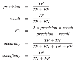
Recall that there are many metrics to evaluate a classifier. We will use AUC as the metrics for the evaluation of the model. Let us see how does the new model perform. A machine learning program is used to evaluate the model performance on test data.

The new model doesn’t perform that well. The AUC score is around 60% on test data.
We now the workings of a logistic regression model. We now know how does it build classifiers. The AUC score of the classifier is not good. We need to look for better models. In the next post of this series, we will look at cross-validation.