Data Science Simplified Part 10: An Introduction to Classification Models

Webster defines classification as follows:

A systematic arrangement in groups or categories according to established criteria.

The world around is full of classifiers. Classifiers help in preventing spam e-mails. Classifiers help in identifying customers who may churn. Classifiers help in predicting whether it will rain or not. This supervised learning method is ubiquitous in business applications. We take it for granted.

In this blog post, I will discuss key concepts of Classification models.

Classification Categories

Regression models estimate numerical variables a.k.a dependent variables. For regression models, a target is always a number. Classification models have a qualitative target. These targets are also called as categories.

In a large number of classification problems, the targets are designed to be binary. Binary implies that the target will only take a 0 or 1 value. These type of classifiers are called as binary classifiers. Let us take an example to understand this.

Regression models estimate numerical variables a.k.a dependent variables. For regression models, a target is always a number. Classification models have a qualitative target. These targets are also called as categories.

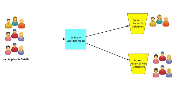
In a large number of classification problems, the targets are designed to be binary. Binary implies that the target will only take a 0 or 1 value. These type of classifiers are called as binary classifiers. Let us take an example to understand this. A bank’s loan approval department wants to use machine learning to identify potential loan defaulters. In this case, the machine learning model will be a classification model. Based on what the model learns from the data fed to it, it will classify the loan applicants into binary buckets:

• Bucket 1: Potential defaulters.
• Bucket 2: Potential non-defaulters.

The target, in this case, will be an attribute like “will_default_flag.” This target will be applicable for each loan applicant. It will take values of 0 or 1. If the model predicts it to be 1, it means that the applicant is likely to default. If the model predicts it to 0, it means that applicant is likely to not default. Some classifiers can also classify the input into many buckets. These classifiers are called as multi-class classifiers.

Linear and Non-Linear Classifiers

Let us say that we want to build a classifier that classifies potential loan defaulters. The features of income and credit rating determines potential defaulters.

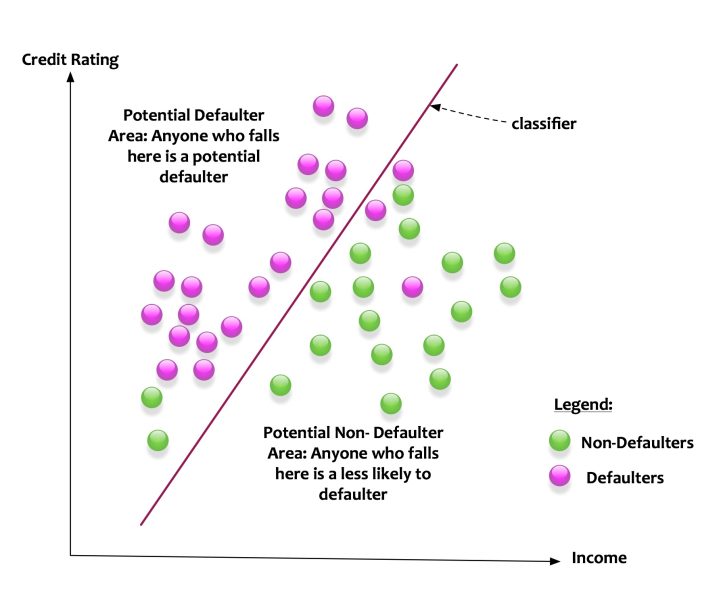
The diagram above depicts the scenario. For simplicity let us say that the feature space is the intersection of income and credit rating. The green dots are non-defaulter and the pink dots are defaulters. The classifier learns based on the input features (income and credit ratings) of data. The classifier creates a line. The line splits the feature space into two parts. The classifier creates a model that classifies the data in the following manner:

• Anyone who falls on the left side of the line is a potential defaulter.
• Anyone who falls on the left side of the line is a potential non-defaulter.

The classifier can split the feature space with a line. Such classifier is called as a linear classifier.

In this example, there are only two features. If there are three features, the classifier will fit a plane that divides the plane into two parts. If there are more than three features, the classifier creates a hyperplane.

This was a simplistic scenario. A line or a plane can classify the data points into two buckets. What if the data points were distributed in the following manner:

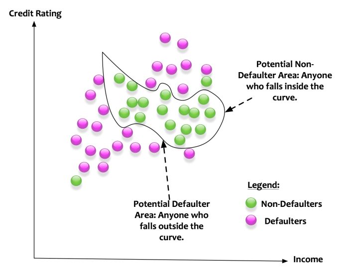
Here a linear classifier cannot do its magic. The classifier needs carve a curve to classify between defaulters and non-defaulters. Such kind of classifiers is called as non-linear classifiers.

There a lot of algorithms that can be used to create classification models. Some algorithms like logistic regression are good linear classifiers. Others like Neural Networks are good non-linear classifiers.

The intuition of the classifier is the following:

Divide the feature space with a function (linear or non-linear). Divide it such that one part of the feature space has data from one class. The other part of the feature space has data from other class

We have an intuition of how classifiers work. How do we measure whether a classifier is doing a good job or not? Here comes the concept of the confusion matrix.

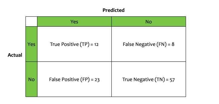
Let us take an example to understand this concept. We built a loan-defaulter classifier. This classifier takes input data, trains on it and following is what it learns.

• The classifier classifies 35 applicants as defaulters.
• The classifier classifies 65 applicants as non-defaulters.

Based on the way classifier has performed, four more metrics are derived:

1. From those classified as defaulters, only 12 were actual defaulters. This metric is called True Positive (TP).
2. From those classified as defaulters, 23 were actual non-defaulters. This metric is called False Positive (FP).
3. From those classified as non-defaulters, only 57 were actual non-defaulters. This metric is called True Negative (TN).
4. From those classified as non-defaulters, 8 were actual defaulters. This metric is called False Negative (FN).

These four metrics can be tabulated in a matrix called as The Confusion Matrix.

From these four metrics, we will derive evaluation metrics for a classifier. Let us discuss these evaluation metrics.

Accuracy:

Accuracy measures how often the classifier is correct for both true positives and true negative cases. Mathematically, it is defined as:

Accuracy = (True Positive + True Negative)/Total Predictions.

In the example, the accuracy of the loan-default classifier is: (12+57) / 100 = 0.69 = 69%.

Sensitivity or Recall:

Recall measures how many times did the classifier get the true positives correct. Mathematically, it is defined as:

Recall = True Positive/(True Positive + False Negative)

In the example, the recall of the loan-default classifier is: 12/(12+8) = 0.60 = 60%.

Specificity:

Specificity measure how many times did the classifier get the true negatives correct. Mathematically, it is defined as:

Specificity = (True Negative)/(True Negative + False Positive)

In the example, the specificity of the loan-default classifier is: 57/(57+23) = 0.7125 = 71.25%.

Precision:

Precision measures off the total predicted to be positive how many were actually positive. Mathematically, it is defined as:

Precision = (True Positive)/(True Positive + False Positive)

In the example, the precision of the loan-default classifier is: 12/(12+23) = 0.48 = 48%.

These are a lot of metrics. On which metrics should we rely upon? This question very much depends on the business context. In any case, one metrics alone will not give a full picture of how good the classifier is. Let us take an example.

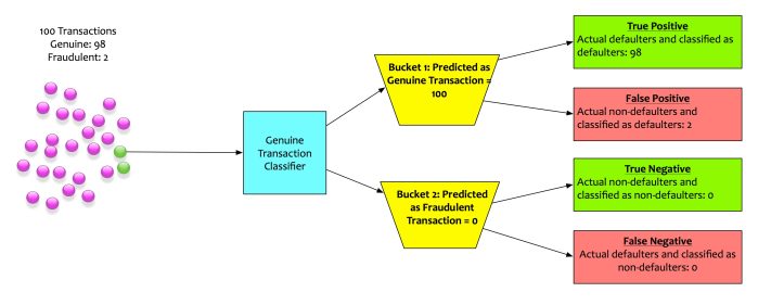
We built a classifier that flags out fraudulent transactions. This classifier determines whether a transaction is genuine or not. Historical patterns shows that there are two fraudulent transaction for every hundred transactions. The classifier we built has the following confusion matrix.

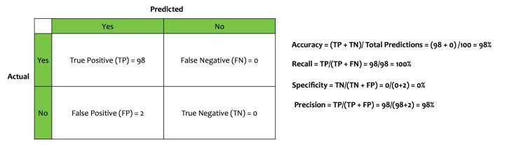
• The Accuracy is 98%
• The Recall is 100%
• Precision is 98%
• Specificity is 0%

If this model is deployed based on the metrics of accuracy, recall, and precision, the company will be doomed for sure. Although the model is performing well, it is, in fact, a dumb model. It is not doing the very thing that it is supposed to do i.e. flag fraudulent transactions. The most important metrics for this model is specificity. Its specificity is 0%.

Since, a single metric cannot be relied on for evaluating a classifier, more sophisticated metrics are created. These sophisticated metrics are combinations of all the above metrics. A few key ones are explained here.

F1 Score:

F1-score is the harmonic mean between precision and recall. The regular mean treats all values equally. Harmonic mean gives much more weight to low values. As a result, the classifier will only get a high F1 score if both recall and precision are high. It is defined as:

F1 = 2x(precision x recall)/(precision + recall)

Receiver Operating Characteristics (ROC) and Area Under Curve (AUC):

Receiver Operating Characteristics a.k.a ROC is a visual metrics. It is a two-dimensional plot. It has False Positive Rate or 1 — specificity on X-axis and True Positive Rate or Sensitivity on Y-axis.

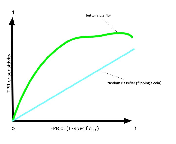
In the ROC plot, there is a line that measures how a random classifier will predict TPR and FPR. It is straight as it has an equal probability of predicting 0 or 1.

If a classifier is doing a better job then it should ideally have more proportion of TPR as compared to FPR. This will push the curve towards the north-west.

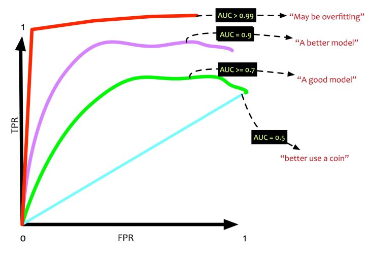
Area Under Curve (AUC) is the area that the ROC curve. If AUC is 1 i.e 100%, it implies that it is a perfect classifier. If the AUC is 0.5 i.e. 50%, it implies that the classifier is no better than a coin toss.