
I thought I would follow on my first blog posting with a follow-up on a claim in the post that going returns followed a truncated Cauchy distribution in three ways. The first way was to describe a proof and empirical evidence to support it in a population study. The second was to discuss the consequences by performing simulations so that financial modelers using things such as the Fama-French, CAPM or APT would understand the full consequences of that decision. The third was to discuss financial model building and the verification and validation of financial software for equity securities.
At the end of the blog posting is a link to an article that contains both a proof and a population study to test the distribution returns in the proof.
The proof is relatively simple. Returns are the product of the ratio of prices times the ratio of quantities. If the quantities are held constant, it is just the ratio of prices. Auction theory provides strategies for actors to choose a bid. Stocks are sold in a double auction. If there is nothing that keeps the market from being in equilibrium, prices should be driven to the equilibrium over time. Because it is sold in a double auction, the rational behavior is to bid your appraised value, its expected value.
If there are enough potential bidders and sellers, the distribution of prices should converge to normality due to the central limit theorem as the number of actors becomes very large. If there are no dividends or liquidity costs, or if we can ignore them or account for them separately, the prices will be distributed normally around the current and future equilibrium prices.
Treating the equilibrium as (0,0) in the error space and integrating around that point results in a Cauchy distribution for returns. To test this assertion a population study of all end-of-day trades in the CRSP universe from 1925-2013 was performed. Annual returns were tested using the Bayesian posterior probability and Bayes factors for each model.
For those not used to Bayesian testing, the simplest way to think about it would be to test every single observation under the truncated normal or log-normal model versus the truncated Cauchy model. Is a specific observation more likely to come from one distribution or another? A probability is assigned to every trade. The normal model was excluded with essentially a probability of zero of being valid.
Bayesian probabilities are different from Frequentist p-values. Frequentist p-values are the probability of seeing the data you saw given a null hypothesis is true. A Bayesian probability does not assume a hypothesis is true; rather it assumes the data is valid and assigns a probability to each hypothesis that it is true. It would provide a probability that data is normally distributed after truncation, log-normally distributed, and Cauchy distributed after truncation. The probability that the data is normally distributed with truncation is less than one with eight million six hundred thousand zeros in front of it when compared to the probability it follows a truncated Cauchy distribution.
That does not mean the data follows a truncated Cauchy distribution, although visual inspection will show it is close; it does imply that a normal distribution is an unbelievably poor approximation. The log-normal was excluded as its posterior didn’t integrate to one because it appears that the likelihood function would only maximize if the variance were infinite. Essentially, the uniform distribution over the log-reals would be as good an estimator as the log-normal.
To understand the consequences, I created a simulation of one thousand samples with each sample having ten thousand observations. Both were drawn from a Cauchy distribution, and a simple regression was performed to describe the relationship of one variable to another.
The regression was performed twice. The method of ordinary least squares (OLS) was used as is common for models such as the CAPM or Fama-French. A Bayesian regression with a Cauchy likelihood was also created, and the maximum a postiori (MAP) estimator was found given a flat prior.
Theoretically, any model that minimizes a squared loss function should not converge to the correct solution, whether statistical or through artificial intelligence. Instead, it should slowly map out the population density, though with each estimator claiming to be the true center. The sampling distribution of the mean is identical to the sampling distribution of the population.
Adding data doesn’t add information. A sample size of one or ten million will result in the same level of statistical power.
SIMULATIONS
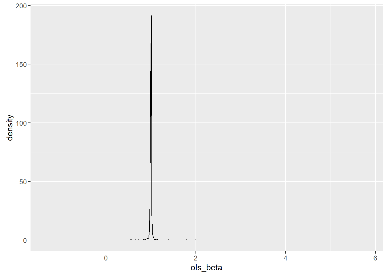
To see this, I mapped out one thousand point estimators using OLS and constructed a graph of it estimating its shape using kernel density estimation.
The sampling distribution of the Bayesian MAP estimator was also mapped and is seen here.
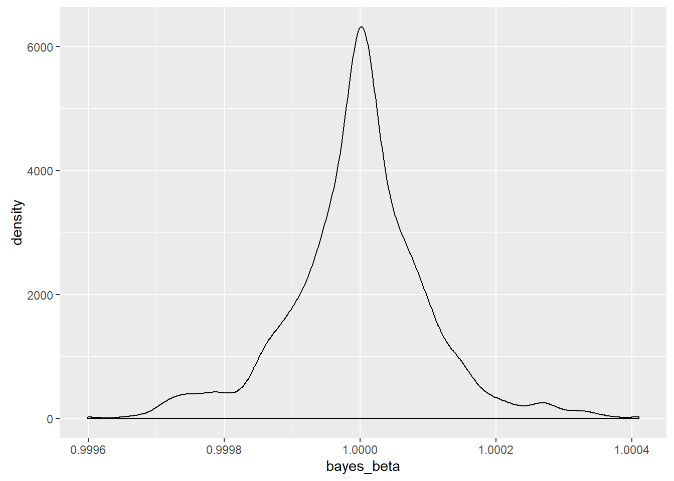
For this sample, the MAP estimator was 3,236,560.7 times more precise than the least squares estimator. The sample statistics for this case were
## ols_beta bayes_beta
## Minimum. : -1.3213 0.9996
## 1st Quarter.: 0.9969 0.9999
## Median : 1.0000 1.0000
## Mean : 1.0030 1.0000
## 3rd Quarter.: 1.0025 1.0001
## Maximum : 5.8004 1.0004
The range of the OLS estimates was 7.12 units wide while the MAP estimates had a range of 0.0008118. MCMC was not used for the Bayesian estimate because of the low dimensionality. Instead, a moving window was created that was designed to find the maximum value at a given scaling and to center the window on that point. The scale was then cut in half, and a fine screen was placed over the region. The window was then centered on the new maximum point, and the scaling was again halved for a total of twenty-one rescalings. While the estimator was biased, the bias is guaranteed to be less than 0.00000001 and so is meaningless for my purposes.
With a true value for the population parameter of one, the median of both estimators was correct, but the massive level of noise meant that the OLS estimator was often far away from the population parameter on a relative basis.
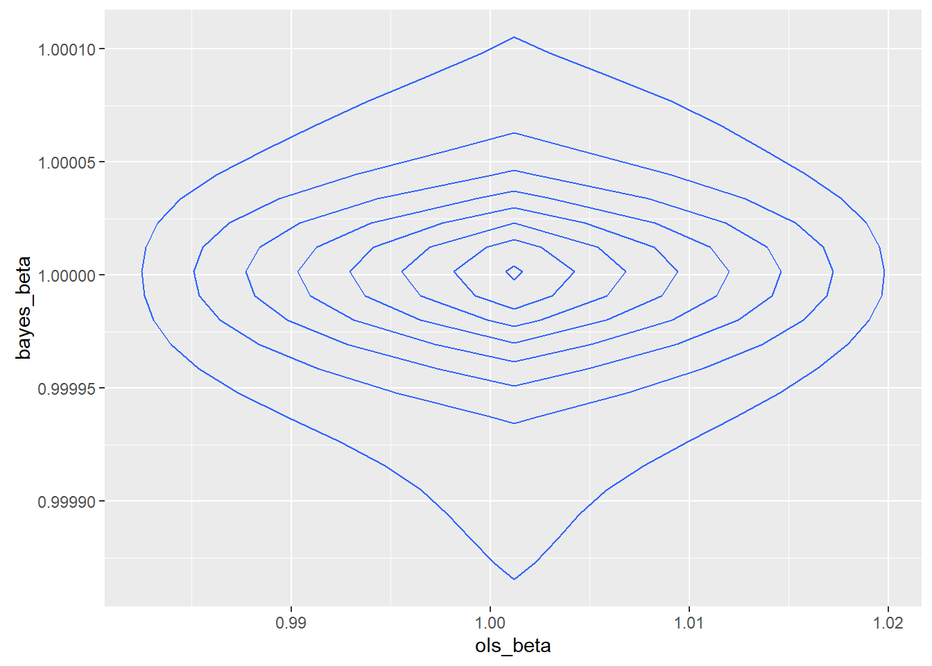
I constructed a joint sampling distribution to look at the quality of the sample. It appeared from the existence of islands of dense estimators that the sample chosen might not be a good sample, though we do not know if the real world is made up of good samples.
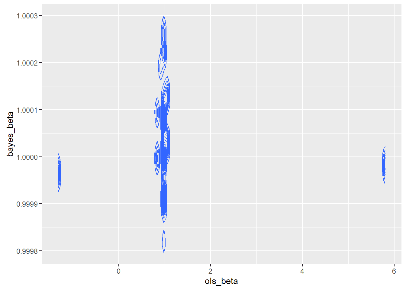
I zoomed in because I was concerned about what appeared to be little islands of probability.
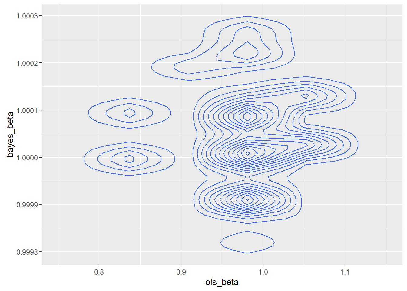
To test the impact of a possibly unusual sample, I drew a new sample of the same size with a different seed.
The second sample was better behaved, though not so well behaved that a rational programmer would consider using least squares. The relative efficiency of the MAP over OLS was 366,981.6. In theory, the asymptotic relative efficiency of the MAP over OLS is infinite. The joint density was
The summary statistics are
## ols_beta bayes_beta
## Mininum : 0.1906 0.9994
## 1st Quarter: 0.9972 1.0000
## Median : 1.0000 1.0000
## Mean : 1.0004 1.0000
## 3rd Quarter: 1.0029 1.0001
## Maximum : 2.2482 1.0005
A somewhat related question is the behavior of an estimator given only one sample.
The first sample of second set resulted in OLS estimates using R’s LM function,
## ## Call:## lm(formula = y[, 1] ~ 0 + x[, 1])
## ## Residuals:##
Minimum 1Q Median 3Q Max
-1985 -1 0 1 83433
## ## Coefficients:## Estimate Std. Error t value Pr(>|t|) ##
x[, 1] 1.000882 0.008043 124.4 <2e-16 *** ## —
## Signif. codes: 0 ‘***’ 0.001 ‘**’ 0.01 ‘*’ 0.05 ‘.’ 0.1 ‘ ‘ 1## ##
Residual standard error: 837 on 9999 degrees of freedom##
Multiple R-squared: 0.6077, Adjusted R-squared: 0.6076 ##
F-statistic: 1.549e+04 on 1 and 9999 DF, p-value: < 2.2e-16
while the Bayesian parameter estimate was 1.000019 and a posterior density for β as appears in the below figure.
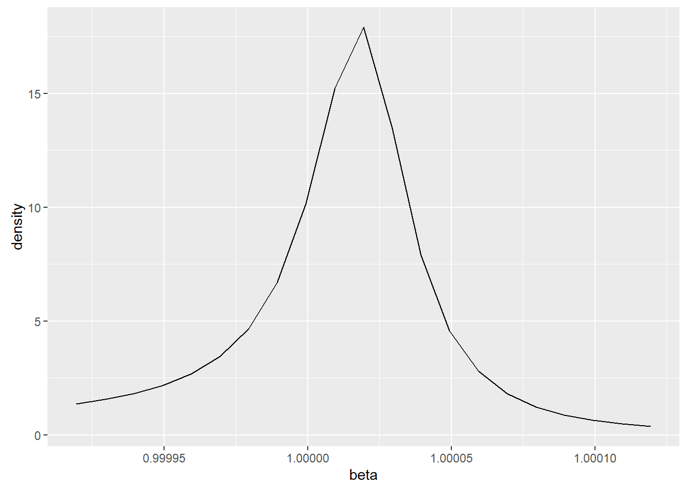
Specific Bayesian intervals were not calculated.
Although the residuals are approximately equal as the coefficients are approximately equal, the residuals have a sample standard deviation of 837, but an interquartile range of 2.04. Based on the assumption of a Cauchy distribution, there were no outliers or very few depending on how one categorized something as an outlier. Based on the assumption of a normal distribution roughly twenty percent of the residuals are outliers.
Just looking for statistical significance won’t provide warnings that something may be amiss.
Model Building
So, if models like the CAPM, APT or Fama-French do not follow using a Bayesian method of model construction, what could work?
The answer would be to go back to first principles. What things should impact returns and scaling?
One of the simplest and most obvious is the probability of bankruptcy, where bankruptcy is defined as the total loss shares by a court for the existing shareholders. Ignoring the causes of bankruptcy for a moment, if π(B) is the probability of bankruptcy, then the required return should be such that
dμ/dπ(B)>0.
Furthermore, since the variance of a Bernoulli trial maximizes at fifty percent, then the scale parameter should grow no less fast than the change in the scaling of the Bernoulli trial. If bankruptcy risk went from one percent to two percent, one would expect the scale parameter of the stock to go up no less than the increase in standard deviation for the risk in the underlying cash flow.
The author previously tested seventy-eight models of bankruptcy against a variety of fundamental and economic variables. Two of the models had approximately fifty-three percent and forty-seven percent of the posterior probability, while the remaining seventy-six model’s posterior probability summed to around one in one hundred and twenty-fifth of a percent.
These models of bankruptcy were highly non-linear, so a curved geometry in high dimensions is likely to be found in this narrow case.
To understand why, consider the accounting measure of current assets – current liabilities. Most bankruptcies are due to a cash crisis. Enron was still profitable under GAAP well after entering into bankruptcy.
However, this gap may indicate different bankruptcies risks at different levels, especially considering that other variables may interact with it. For example, a firm with just a small cushion of current assets over current liabilities will probably not have a particularly high risk of sudden failure. What about the other two extremes?
For a firm to carry a large negative gap, some other firm has to be underwriting their liabilities. That would usually be a bank. If a bank is underwriting their liabilities, then the bank has adjudged their risk of loss to be small. It implies that the bank has sufficient confidence in the business model to extend credit without the immediate ability to repay. Further, because banks love to place a mountain of protective covenants, the management of the bank is likely constrained from engaging in shenanigans as it is being monitored and prohibited from doing so.
On the other side of the gap, a large amount of current resources may have an indeterminate meaning. Other variables would need to be consulted. Is nobody buying their inventory? Is it a month before Black Friday and they have just accumulated an enormous inventory for a one day sale? Are they conserving cash expecting very bad times in the immediate future? Is the management just overly conservative?
The logic also could vary by firm. Some economic or accounting variables are of no interest to a firm. An electrical utility has no way to incentivize or materially influence the bulk of its demand. The weather is of far greater importance. It cannot control its revenue. A jeweler, on the other hand, may have a substantial influence on its revenue through careful pricing, marketing, and judicious credit terms. Revenue may have a very different meaning to a jeweler. Likewise, some products do not depend on economic circumstances to determine the amount purchased. Examples of this include goods such as toilet paper or aspirin. Model construction should involve thinking.
Imagine a set of two factors whose expected bankruptcy rate is a paraboloid. Will your neural network detect the mapping of those features onto returns or a decision function? What if the top of the paraboloid has extra bends in it? A good method to start the validation process is to simulate the conditions where the model is likely to have difficulties.
Ex-ante validation of mapping factors to decisions for neural networks should be more about the ability to map from a geometry onto another geometry. The mean-variance finance models were nice because they implied a relatively low dimensionality with linear, independent relationships.
The alternative test models should not be uncorrelated as there is high correlation among variables in finance. Rather, it should be a test of correlated but incorrect geometries.
Large-scale model building often implies grabbing large amounts of data with many variables and doing automated model selection. I have no argument with that, but I do recommend two things. First, remember that accounting and economic data are highly correlated by design. Second, remember that simple linear relationships may not may logical sense from a first principles perspective so be highly skeptical.
For the first, a handful of variables contain nearly all the independent information. The Pearson correlation among accounting entries in the COMPUSTAT universe range from .6 to .96 depending on the item. Adding variables doesn’t add much information.
For the second case, a simple mapping of believed associations and how they would impact mergers, bankruptcies, continued operations and dividends would be useful as well as how they would likely interact with each other to determine a rational polynomial or other function as the form.
As this is being done as software, that software should undergo a verification and validation (V&V) process.
Verification and validation differ slightly from the simple testing of software code in a couple of ways. If I write code and test it, I am not performing either verification or validation automatically.
In an ideal world, the individual performing the V&V would be independent of the person writing the code and of the person representing the customer, although that is an ideal. It is an extra cognitive step. The verifier is determining whether or not the software meets requirements. Simplified, is the software solving the problem intended to be solved? It has happened, more than once in the history of software development, that the designers and builders of software have interpreted communications from a customer differently than the customer intended. In the best of worlds, quite a bit of time is spent communicating between customer and builder clarifying what both parties are really talking about.
Validation, on the other hand, is a different animal. It is a check to determine if the proposed solution is a valid solution to the problem. It is here where financial economics and data science may get a bit sticky. Much depends upon how the question was asked. Saying “I used an econophysics approach to create the order entry system,” does not answer the question. Answering with “well, I cross-validated it,” also doesn’t answer the question of “does it solve the actual problem.” The cross-validation procedure, itself, is subject to V&V.
Are you solving the problem the customer feels needs to be addressed and is your solution a valid solution?
Imagine a human resource management system for pit traders that is designed to determine which employee will be on the floor. Behavioral economics notes that individuals that have lost money behave differently than those who were recently profitable. The goal is to create a mechanism to detect which traders should be on the floor. Mean-variance finance would imply that such an effect shouldn’t exist. The behavioral finance observation has been supported in the literature. The question is what theory to use, how to verify the solution and validate it.
The answer to that depends entirely on what the customer needs. Do they need to minimize the risk of any loss? Maximize dollar profits? Maximize percentage profits? Produce profits relative to some other measure? As behavioral finance is descriptive and not prescriptive, it may be the case that replacement traders will not improve performance. When considering which mechanism and measurement system to adopt, the question has to always go back to the question being asked of the data scientist.
The proposed calculus in the prior blog posting adds a new layer to mathematical finance. In it, there is a claim that returns, given that the firm would remain a going concern and ignoring dividends and liquidity costs, would converge to a truncated Cauchy distribution. That is quite a bit at odds with the standard assumption of a normal distribution being present or a log-normal distribution being present, but certainly in the literature since the 1960s.
Nonetheless, the assumption of normality or log-normality is built on models that presume that the parameters are known. If the assumption that the markets know the parameters is dropped, then a different result follows.
The primary existing models haven’t passed validations studies. The author believes it is due to the necessary assumption in the older calculus that the parameters were known. Dropping that assumption will create validation issues as everyone is on new ground. Caution is advised.
Future Posts
In my upcoming blog posts, I am going to cover the logarithmic transformation. It isn’t a free lunch to use. I am also going to cover additional issues with regression. However, my next blog posting will be on sex and the math of the stock market.
There is a grave danger in blind, large-scale analysis of ignoring the fact that we are modeling human behavior. Unfortunately, it is an economic discussion so it won’t be an interesting article on sex. Sex and food are simpler to discuss as low-level toy cases than questions of power or money. For reasons that are themselves fascinating, people spend hours or days analyzing what stock to pick, but minutes to figure out who to potentially have children with.
The entire reason managers are taught numerical methods is to prevent gut decisions. Leadership isn’t everything, management matters.
It takes leadership to convince people to climb a heavily defended hill, possibly to their death or dismemberment. No one will respond to a person with a clipboard letting them know they will get three extra points on his or her quarterly review if he or she takes the hill. They will follow a leader to certain death to defend their nation.
On the other hand, leadership will not get food, ammunition, clothing or equipment to their encampment on time and in the right quantities at the correct location. Only proper management and numerical analysis can do that. Data science can inform management decisions, so it is best to remember we are not, automatically, a logical species.
Also, before everyone runs for the door on the Fama-French model, I will present a defense of it that I hope will serve as both a warning and a cause to look deeper into their model. Fama and French were responding to the CAPM, not replacing it.
Up next, sex, data science, and the stock market…
For empirical verification of the above proof see the article at the Social Science Research Network.
References
Curtiss, J. H. (1941). On the distribution of the quotient of two chance variables. Annals of Mathematical Statistics, 12:409-421.
Davis, H. Z. and Peles, Y. C. (1993). Measuring equilibrating forces of financial ratios. The Accounting Review, 68(4):725-747.
Grice, J. S. and Dugan, M. T. (2001). The limitations of bankruptcy prediction models: Some cautions for the researcher. Review of Quantitative Finance and Accounting, 17:151-166. 10.1023/A:1017973604789.
Gurland, J. (1948). Inversion formulae for the distribution of ratios. The Annals of Mathematical Statistics, 19(2):228-237.
Harris, D. E. (2017). The distribution of returns. The Journal of Mathematical Finance, 7(3):769-804.
Hillegeist, S. A., Keating, E. K., Cram, D. P., and Lundstedt, K. G. (2004). Assessing the probability of bankruptcy. Review of Accounting Studies, 9:5-34.
Jaynes, E. T. (2003). Probability Theory: The Language of Science. Cambridge University Press, Cambridge.
Marsaglia, G. (1965). Ratios of normal variables and ratios of sums of uniform variables. Journal of the American Statistical Association, 60(309):193-204.
Nwogugu, M. (2007). Decision-making, risk and corporate governance: A critique of methodological issues in bankruptcy/recovery prediction models. Applied Mathematics and Computation, 185:178-196.
Sen, P. K. (1968). Estimates of the regression coefficient based on Kendall’s tau. Journal of the American Statistical Association, 63(324):1379-1389.
Shepard, L. E. and Collins, R. A. (1982). Why do farmers fail? Farm bankruptcies 1910-1978. American Journal of Agricultural Economics,64(4):609-615.
Sun, L. and Shenoy, P. P. (2007). Using Bayesian networks for bankruptcy prediction: Some methodological issues. Computing, Artificial Intelligence and Information Management, 180:738-753.