
It’s been said that Data Scientist is the “sexiest job title of the 21st century.” This is because of one main reason that there is a humongous amount of data available as we are producing data at a rate as never before. With the dramatic access to data, there are sophisticated algorithms present such as Decision trees, Random Forests etc. When there is a humongous amount of data available, the most intricate part is to select the correct algorithm to solve the problem. Each model has its own pros and cons and should be selected depending on the type of problem at hand and data available.
Decision Trees:
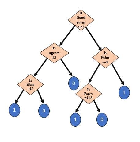
The aim of this blog post is to discuss one of the most widely used Machine Learning algorithm: “Decision Trees”. As the name suggests, it uses a tree-like model to make decisions as shown in below figure. Decision Tree is drawn upside down with its root at the top. A question is asked at every node based on which decision tree splits into branches. The end of the tree which doesn’t split further is called as Leaf.
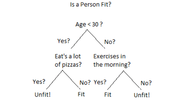
Decision Trees can be used for classification as well as regression problems. That’s why there are called as Classification or Regression Trees(CART). In the above example, a decision tree is being used for a classification problem to decide whether a person is fit or unit. The depth of the tree is referred to length of the tree from root node to leaf.
For basics of the decision tree, click here.
Have you ever given the thought that if there are so many sophisticated algorithms available such as neural networks which are better in terms of parameters such as accuracy then why decision trees are one of the most widely used algorithms?
The biggest advantage of Decision Trees is interpretability. Let’s talk about neural networks to understand this. To make the concept of neural network easy to understand, let’s consider the neural network as “Black Box”. The set of input data is given to the black box and it produces the output corresponding to the input data set. Now, What’s inside the black box? Black Box consists of a computational unit which consists of several hidden layers depending on the intricacy of problem. Also, a large amount of data set is required to train these hidden layers. With the increased no. of hidden layers, there is a significant increase in the complexity of neural networks. It becomes very hard to interpret the output of neural networks in such cases. That’s where lies the importance of decision trees. Decision Trees interpretability helps the humans to understand what’s happening inside the black box? This can help significantly to improve the performance of neural networks in terms of several parameters such as accuracy, avoiding the overfitting etc.
Another advantage of Decision Trees includes a nonlinear relationship between the parameters doesn’t affect the tree performance, Decision implicitly performs the feature selection and minimal effort for data cleaning.
As already discussed, every algorithm has it’s pros and cons. Disadvantages of Decision Trees include poor performance if the decision tree is overfitted to data and could not generalize well. Decision trees can be unstable for small variations of data. So, this variation should be reduced by methods such as bagging, boosting etc.
If you have used ever implemented decision trees: Have you ever thought what’s happening in the background when you implement a decision tree using sci-kit learn in Python? Let’s understand the nitty-gritty of decision trees i.e. various functions such as train test split, checking the purity of data, classification of data, calculating the overall entropy of data etc. that runs in the background. Let’s understand the concept of the decision tree by implementing it from scratch i.e. with the help from numpy and pandas (without using skicit learn).
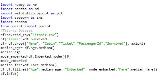
Here, I am using Titanic dataset to build a decision tree. Decision tree needs to be trained to classify whether the passenger is dead or survived based on parameters such as Age, gender, Pclass. Note that titanic data set contains various variables such as passenger name, address etc which are dropped because they are just identifiers and doesn’t add value to the decision tree. This process is formally called “Feature Selection.”
The first step toward building the ML algorithm is data cleaning. It is one of the most important step because the model build on unformatted data can affect the performance of the model significantly. I am going to use the Titanic data set to build the decision tree. The aim of this model is to classify the passengers as survived or not based on information given. The first step is to load the data set, clean it. Cleaning of data consists of 2 steps:
Dropping the variables which are of least importance in deciding. In Titanic dataset columns such as name, cabin no. ticket no. is of least importance. So, they have been dropped.
Fill in all the missing values i.e. replace NA’s with the most suitable central tendency. All the NA’s are replaced with Mean in case of continuous variables and mode in case of categorical variables. Once the data is clean, we will try to build the helper functions which will help us to write the main algorithm.
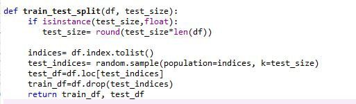
Train-Test Split:
We are going to divide the data set into 2 sets i.e. train data set and test data set. I have kept the train test split ratio as 80:20. However, this could be different. The best practice is to keep the test data set small as compared to the train data set depending on the size of the data set. But the test should not be so small that it is not representative of the population
In the case of large data sets, the data set is divided into 3 categories: Training Data Set, Validation Data Set, Test Data Set. Train data is used to train the model, validation data set is used to tune the model in terms of parameters such as accuracy, overfitting. Once the model is verified for the optimal accuracy, it can be used for testing.
Check Data Purity and classify:
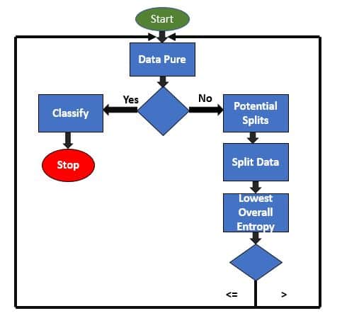
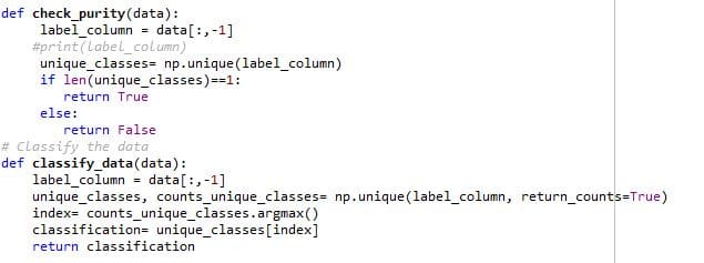
As shown in the block diagram, Data Pure function check the data set for its purity i.e. if the data set contains only one species of flower. If so, it will classify the data. If the data sets contain different species of flowers, it will try to ask the questions which can accurately segregate the different species of flowers. It is done by implementing functions such as potential splits, split data, calculate the overall entropy. Let’s understand each of them in detail.
Potential Splits Function:
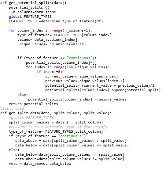
Potential splits function gives all the possible splits for all of the variables. In Titanic dataset, there are 2 kinds of variables Categorical and Continuous. Both the types of variables are handled in a different way.
For a categorical variable, each unique value is taken as possible split. Let’s take the example of gender. Gender can only take up 2 values either male or female. Possible splits are male and Female. The question will be simple: Is Gender == “Male”. In this way, the decision tree can segregate the population based on Gender.
Since the continuous variable can take on any value. So, the potential split can be exactly in the midpoint of two values in the data set. Let’s understand this with the help of “Fare” Variable in Titanic data set. Suppose, Fare = {10,20,30,40,50}. Potential Splits for Fare will be: 15, 25,35,45. If we ask the question “If Fare <=25”, we can segregate the data effectively. Since Fare variable can take up any value between 10 to 50 in the above case, we can’t deal the continuous variable in the same way as a categorical variable.
Once potential split function gives all the potential splits for all the variables. Split data function is used to split data based on each and every potential split. It divides the data into 2 halves, data above and data below. Entropy is calculated for each split.
Measure of Impurity:
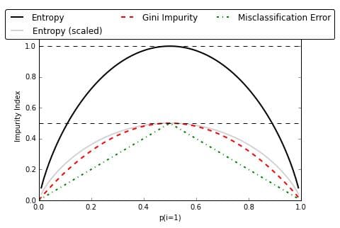
There are two methods to measure the impurity: Gini Impurity and Information Gain Entropy. Both the methods work the same and the selection of impurity measure has little impact on the performance of the decision tree. But Entropy is computationally expensive since it deals with the logarithmic functions. This is the main reason for the large-scale use of Gini Impurity over Information Gain Entropy. Below are formulae for both:
- Gini: Gini(E)= 1-∑j=1(pj2)
- Entropy: H(E)=−∑cj=1(pjlogpj)
I have used Information Gain Entropy as a measure of impurity. You can use either of them, as both give pretty much same results specifically in case of CART analytics as shown in below figure. Entropy in simpler terms is the measure of randomness or uncertainty. For each potential split, entropy will be calculated. The best potential split will be the one with the lowest overall entropy. This is because of lower the entropy, lower the uncertainty and hence more the probability.
Refer to below link for the comparison between the two methods of impurity measure:
https://github.com/rasbt/python-machine-learning-book/blob/master/f…
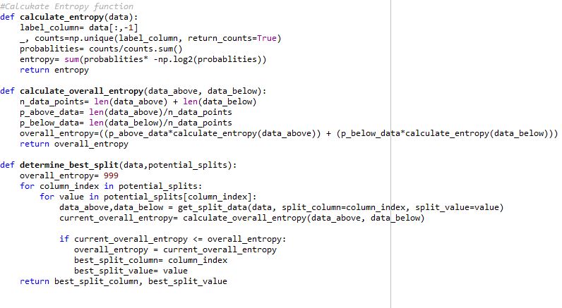
To calculate entropy in titanic dataset example, calculate entropy and calculate overall entropy functions are used. The functions are defined based on the equations explained above. Once the data is split into two halves by split data function, entropy is calculated for each and every potential split. The potential split with lowest overall entropy is selected as best split with the help of determining the best split function
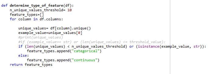
Determine type of feature:
Determine type of feature functions determine whether a type of feature is categorical or continuous. There are 2 criteria’s for the feature to be called as categorical, first if the feature is of data type string and second, the no. of categories for the feature is less than 10. Otherwise, the feature is said to be continuous.
Determine type of feature determines whether the function is categorical or not based on the above criteria which act as input to a potential split function. This is because potential split has a different way to handle categorical and continuous data as discussed in the potential split function above
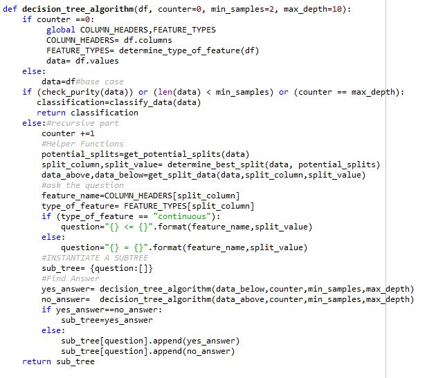
Decision Tree Algorithm:
Since we have built all the helper functions, it’s now time to build the decision tree algorithm.
Target Decision Tree should look like:
As shown in the above diagram, Decision Tree consists of several sub-trees. Each sub-tree is a dictionary where “Question” is key of the dictionary and there are two answers corresponding to each question i.e. Yes answer and No answer.
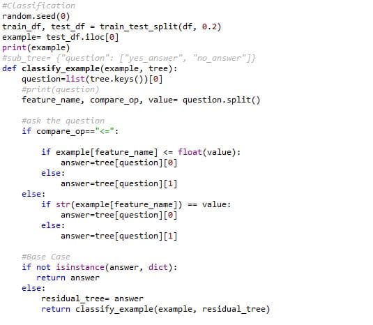
Representation of sub-tree is given as follows:
sub_tree= {“question”: [“yes_answer”, “no_answer”]}
Decision Tree Algorithm is the main algorithm which is used to train the model with the help of helper functions which we built previously. Firstly, Train Test Split function is called which divides the data set into train data and test data. Once the data is split, Data Pure and Classify function is called to check the purity of data and classify the data based on purity. The potential Split function gives all the potential splits for all variables. Overall Entropy is calculated for each potential split and eventually, potential split with lowest overall entropy is selected and split data function splits the data into two parts. In this way, the subtree is built and a series of sub-trees constitutes our target Decision Tree.
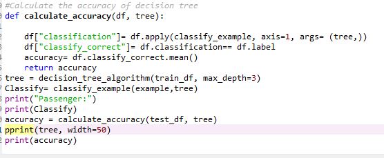
Once the model is trained on training dataset, the performance of Decision Tree is verified on the test data set with the help of classifying function. The performance of the model is measured in terms of accuracy by calculating accuracy function. The performance of the model can be improved by pruning the tree based on the max depth of the tree. The accuracy of the model is coming out to be 77%.
Original Article Published here Building Blocks of Decision Tree