Bootstrap aggregating (bagging), is a very useful averaging method to improve accuracy and avoids overfitting, in modeling the time series. It also helps stability so that we don’t have to do Box-Cox transformation to the data.
Modeling time series data is difficult because the data are autocorrelated. In this case, moving block bootstrap (MBB) should be preferred because MBB resamples the data inside overlapping blocks to imitate the autocorrelation in the data. If the length of a time series, n, and the block size l, the number of overlapping blocks are found as below:

What we mean by overlapping block is that observation 1 to l would be block 1, observation 2 to l+1 would be block 2, etc. We should use a block size for at least two years(l=24) for monthly data because we have to be certain whether there is any remaining seasonality in the block.
From these n-l+1 blocks, n/l blocks will be selected randomly and they will be gathered in order, to build the bootstrap observations. The time series values can be repetitive in different blocks.
This bootstrap process would be exercised to the remainder component after the time series decomposition. If there is seasonality it is used the stl function(trend, seasonal, remainder) otherwise the loess function(trend, remainder) is chosen for the decomposition. It should not be forgotten that the data has to be stationary in the first place.
Box-Cox transformation is made at the beginning but back-transformed at the end of the process; as we mentioned before, when we do average all the bootstrapped series, which is called bagging, we could handle the non-stability data problem and improve accuracy compared to the original series.
As we remembered from the previous two articles, we have tried to model gold prices per gram in Turkey. We have determined the ARIMA model the best for forecasting. This time, we will try to improve using the bagging mentioned above.
In order to that, we will create a function that makes bootstrapping simulations and builds the prediction intervals we want. We will adjust the simulation number, model, and confidence level as default. We will use the assign function to make the bagged data(simfc) as a global variable, so we will able to access it outside the function as well.
#Simulation functionlibrary(purrr)library(forecast)sim_forecast <- function(data, nsim=100L, h, mdl=auto.arima, level=95){ sim <- bld.mbb.bootstrap(data, nsim) h <- as.integer(h) future <- matrix(0, nrow=nsim, ncol=h) future <- sim %>% map(function(x){simulate(mdl(x),nsim=h)}) %>% unlist() %>% matrix(ncol = h, nrow = nsim, byrow = TRUE) start < - tsp(data)[2]+1/12 simfc <- structure(list( mean = future %>% colMeans() %>% ts(start = start, frequency = 12), lower = future %>% as.data.frame() %>% map_dbl(quantile, prob = (1-level/100)/2) %>% ts(start = start,frequency = 12), upper = future %>% as.data.frame() %>% map_dbl(quantile, prob = (1-level/100)/2+level/100) %>% ts(start = start,frequency = 12), level=level), class="forecast") assign("simfc",simfc,envir = .GlobalEnv) simfc } |
Because of the averaging part of the bagging, we don’t use the lambda parameter of Box-Cox transformation for the stability of the variance. We can see the forecasting results for 18 months in %95 confidence interval for training set below. We can also change the model type or confidence level if we want.
sim_forecast(train, h=18) Point Forecast Lo 95 Hi 95#Mar 2019 242.3121 215.5464 268.2730#Apr 2019 243.4456 206.4015 274.5155#May 2019 249.9275 216.8712 283.4226#Jun 2019 252.8518 219.7168 283.0535#Jul 2019 259.0699 216.7776 302.4991#Aug 2019 267.2599 219.5771 310.7458#Sep 2019 270.8745 214.1733 324.4255#Oct 2019 272.0894 215.1619 333.2733#Nov 2019 275.5566 213.8802 337.9301#Dec 2019 280.3914 219.2063 349.1284#Jan 2020 291.4792 215.9117 364.1899#Feb 2020 296.3475 221.9117 380.2887#Mar 2020 302.0706 219.0779 399.1135#Apr 2020 304.4595 217.5600 400.7724#May 2020 310.8251 217.5561 420.6515#Jun 2020 315.5942 221.5791 431.9727#Jul 2020 322.4536 220.4798 452.4229#Aug 2020 331.1163 223.3746 465.2015 |
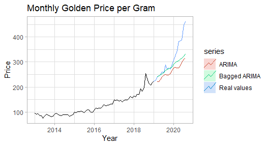
We will create the Arima model as same as we did before and compare it with a bagged version of it in a graph.
arimafc <- train %>% auto.arima(stepwise = FALSE,approximation = FALSE, seasonal = FALSE, lambda = "auto") %>% forecast(h=h,level=95)autoplot(train) + ggtitle("Monthly Golden Price per Gram") + xlab("Year") + ylab("Price") + autolayer(test, series="Real values",PI=FALSE) + autolayer(simfc, series="Bagged ARIMA",PI=FALSE) + autolayer(arimafc, series="ARIMA",PI=FALSE)+ theme_light() |
When we examine the above plot, we can see that the bagged Arima model is smoother and more accurate compared to the classic version; but it is seen that when the forecasting horizon increases, both models are failed to capture the uptrend.
In the below, we are comparing the accuracy of models in numeric. We can easily see the difference in the accuracy level that we saw in the plot. The reason NaN values of the simulated version is that there is no estimation of fitted values(one-step forecasts) in the training set.
#Accuracy comparisonacc_arimafc <- arimafc %>%accuracy(test)acc_arimafc[,c("RMSE","MAPE")]# RMSE MAPE#Training set 9.045056 3.81892#Test set 67.794358 14.87034acc_simu <- simfc %>% accuracy(test)acc_simu[,c("RMSE","MAPE")]# RMSE MAPE#Training set NaN NaN#Test set 54.46326 8.915361 |
Conclusion
When we examine the results we have found, it is seen that bootstrapping simulation with averaging (bagging) improves the accuracy significantly. Besides that, due to the simulation process, it can be very time-consuming.
The original article can be found here.
References
- Forecasting: Principles and Practice, Rob J Hyndman and George Athanasopoulos
- Bagging Exponential Smoothing Methods usingSTL Decomposition and Bo…, Christoph Bergmeira, Rob J Hyndmanb, Jos ́e M Benitez
- Block Bootstrap, Wikipedia
- Bootstrap aggregating, Wikipedia

