Bayesian Machine Learning (Part 8) - DataScienceCentral.com

Bayesian Machine Learning (part-8)

Mean Field Approximation

Have you ever asked a question, why do we need to calculate the exact Posterior distribution ?

To understand the answer the above question, let us go to –

Back to the Basics !

To understand the answer of the above question, I would like you to re-visit our basic Baye’s rule.

Posterior = (Likelihood x Prior) / Evidence

Now to compute the Posterior we have following issues:

If prior is conjugate to likelihood, it is easy to compute the posterior, otherwise not
It is really very hard to compute the evidence of the points

So, what if we try and approximate our posterior!

Will it impact our results? .. let us check out with an example.

Let us suppose we have a probabilistic distribution as shown in the figure:

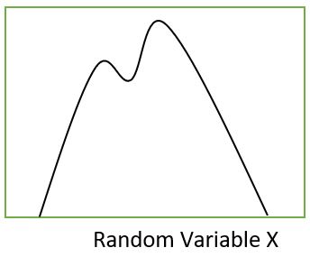
The computation of the exact posterior of the above distribution is very difficult.

Now suppose we try to approximate the above distribution with a gaussian distribution which looks as follows:

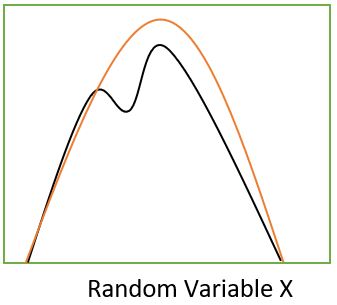
Now from the above figure we can say the error is very small as the gaussian distribution is conveniently satisfying the job. Also, in machine learning problems, we really do not want an exact value of the posterior as far as we can get relative values for decision making.

From the above example we saw that if we have good approximate distribution for the posterior, we are good to go !

The next question arises, how to compute this approximate posterior distribution.

Computing the Approximate Distribution

To compute the approximate distribution, we will have to consider a family of distribution and then we will try to minimize the KL Divergence parameter between the actual posterior and the approximate distribution.

Mathematically speaking,

KL Divergence :

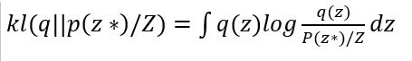
Expanding the above equation, we get :

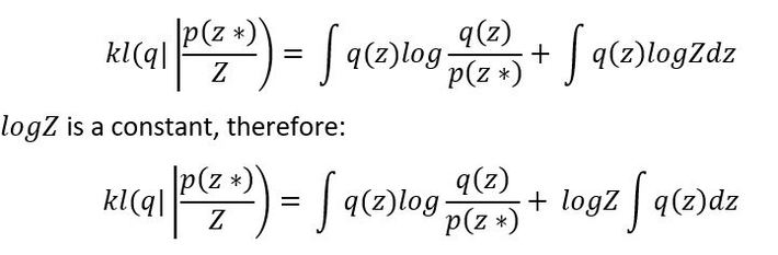
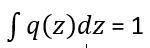
as q(z) is a probabilistic distribution and Log z is a constant for a given data, therefore It does not play a role in differentiation process of KL divergence to minimize the distance between the approximate posterior distribution and the actual distribution.

So, now we will understand a methodology to do this approximation.

Mean Field Approximation

The name suggests a word ‘mean’, we will see the importance of this later in the blog. Another word ‘field’ is basically coming from electromagnetism theory of physics, as this approximation methodology incorporates the impact of nearby neighbors in making the decision, thus incorporating the fields impacts of all neighbors.

So, let us start learning the concept behind this approximation.

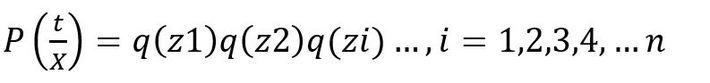
Step 1 : Suppose the posterior distribution has n dimensions, then we will consider total n different distributions to approximate the posterior.

Step 2 : all the n different distributions will be multiplied together to approximate the posterior. The mathematical expression looks as :

Step 3 : now the expression of KL divergence is used to differentiate and minimize the distance between the posterior and approximation. We use coordinate descent method to differentiate the expression, which differentiates the expression w.r.t to one variable, update the expression and then differentiate w.r.t another variable and so on.

Mathematical Derivation

KL divergence expression :

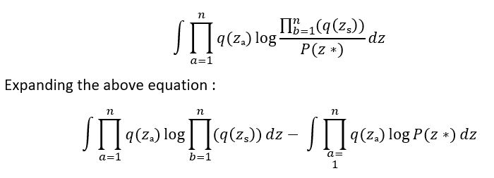
Now, we only need to differentiate w.r.t k, therefore all the dimensions are constant as per coordinate descent.

By taking q(z_k) as common and treating the remain multiplier as a constant and for the second object for P(z*), it becomes as Expected value for the random variable q(z₁)*q(z₂) … q(z_i) where i != k.

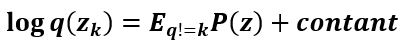
The final expression we get is :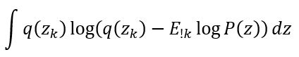

Now, with a little conversion of the equation, it re occurs in form of KL divergence, and to differentiate and equate it to zero means equating the denominator and numerator. The final expression is as follows:

Now because of the mean impact of remaining dimensions results in th most optimal solution of the k^th dimension, we call it mean fields.

Practical understanding

Now, what you just saw may be very scary !!! right ..

Let us take a working example to understand the concept of mean field approximation in more practical manner.

Grey scale image de-noising is a very popular use case of MFVI. It uses 2 concepts – Ising model and approximating the ising model using Mean field approximation. Below are the details:

Ising Model : is a mathematical model of ferromagnetism in statistical mechanics.

Core Idea behind Merging two theories : ferromagnetic substances, at their molecular level can have 2 types of spins – clockwise or anticlockwise. If the spins of all the molecules are same and aligned, the object start behaving as a magnet. The spin of any molecule has a significant impact from its neighboring molecules. This impact varies from substance to substance. Thus it makes the occurrence of the spin for each molecule probabilistic. Ising Model defines this behavior mathematically.

Now, we can consider our image as 2-D substance sheet and can consider every pixel of the image as a molecule. In a binary-image, these pixels can take only 2 values i.e. black and white, analogously -1 and 1. This image can be de-noised by considering the same theory that each pixel will take value as per its neighbor. And so we can apply Ising model to re correct the spins/black-white/-1,+1 values of the image, if we control the neighbor impact property of the image.

Now, the joint probabilistic distribution of the Ising model is impossible to evaluate analytically, thus we use Mean Field Approximation theory to evaluate it.

Example :

I tried this approach on a grey image of a bird by adding a lot of noise to it and tried to retrieve as much as possible from it. Below are my results :

Noisy Image: