
Bayesian Machine Learning (part -6)
Probabilistic Clustering – Gaussian Mixture Model
Continuing our discussion on probabilistically clustering of our data, where we left out discussion on part 4 of our Bayesian inference series. As we have seen the modelling theory of Expectation – Maximization algorithm in part-5, its time to implement it.
So, let’s start!!!
For a better revision, please follow the link :
Remembering our problem
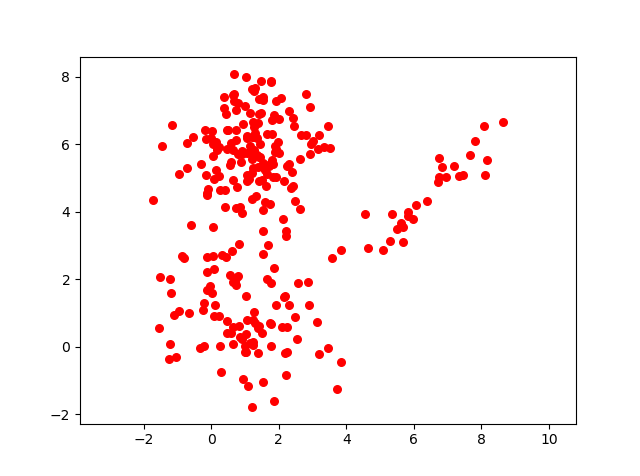
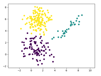
We were having observed data as given in the below picture.
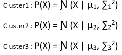
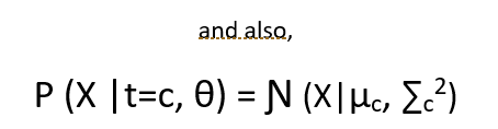
We have assumed there are in total 3 clusters and for each cluster we have defined the Gaussain distribution as follows :
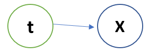
We considered that data came from a Latent variable t who knows which data point belongs to which data point with what probability. The Bayesian model looks like :
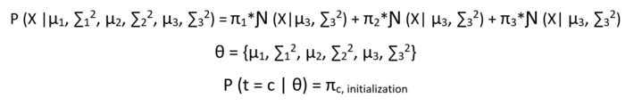
Now the probability of the observed data given the parameters looks like :
The point to note here is that the equation :

Is already in its lower bound form, so no need to apply Jensen’s inequality.
E-Step
As we know the E-step solutions is :
q(t=c) = P(t=c | Xi ., θ)
As we know there are 3 clusters in our case we will need to compute the posterior distribution for our latent carriable t for all the 3 clusters, so, let’s see how to do it.

We will perform the above equation for all the observed data points, for every cluster with respect to every point. So, for example we have 100 observed data points and have 3 clusters, then the matrix of the posterior on the latent variable t is of dimension – 100 x 3.
M-Step
In the M step, we maximize our lower bound variational inference w.r.t θ and we use above computed posterior distribution on our latent variable t as constants. So let’s start,
The equation we need to maximize w.r.t θ and π1 ,π2 , π3 , is:
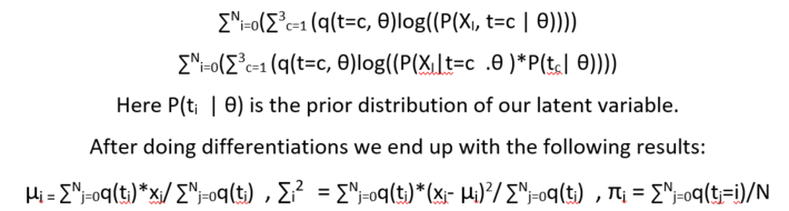
The priors are computed with constraint that every prior >= 0 and sum of all
prior = 1
These E step and M step are iterated a multiple time one after the other, in a fassion that results of E step are used in M step and results of M step are used in E step. Doing this we end the iteration when the loss funtions stops reducing.
The loss funtion is the same function which we are differentiating in the M step.
The result of applying the EM algorithm on the given data set is as below:
So, in this post we saw how we can implement the EM algorithm for probabilistic clustering.
Thanks For Reading !!!