
Bayesian Machine Learning (part – 3)
Bayesian Modelling
In this post we will see the methodology of building Bayesian models. In my previous post I used a Bayesian model for linear regression. The model looks like:
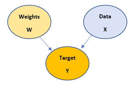
So, let us first understand the construction of the above model:
- when there is an arrow pointing from one node to another, that implies start nodes causes end node. For example, in above case Target node depends on Weights node as well as Data node.
- Start node is known as Parent and the end node is known as Child
- Most importantly, cycles are avoided while building a Bayesian model.
- These structures normally are generated from the given data and experience
- Mathematical representation of the Bayesian model is done using Chain rule. For example, in the above diagram the chain rule is applied as follows:
P(y,w,x) = P(y/w,x)P(w)P(x)
Generalized chain rule looks like: 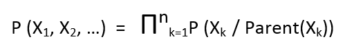
- The Bayesian models are build based upon the subject matter expertise and experience of the developer.
An Example
Problem Statement : Given are three variables : sprinkle, rain , wet grass, where sprinkle and rain are predictors and wet grass is a predicate variable. Design a Bayesian model over it.
Solution:
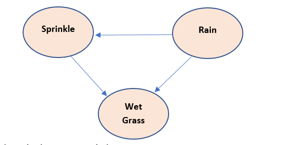
Theory behind above model:
- Sprinkle is used to wet grass, therefore Sprinkle causes wet grass so Sprinkle node is parent to wet grass node
- Rain also wet the grass, therefore Sprinkle causes wet grass so Rain node is parent to wet grass node
- if there is rain, there is no need to sprinkle, therefore there Is a negative relation between Sprinkle and rain node. So, rain node is parent to Sprinkle node
Chain rule implementation is :
P(S,R,W) = P(W/S,R)*P(S/R)*P(R)
Latent Variable Introduction
Wiki definition: In statistics, latent variables (from Latin: present participle of lateo (“lie hidden”), as opposed to observable variables), are variables that are not directly observed but are rather inferred (through a mathematical model) from other variables that are observed (directly measured)
In my words: Latent variables are hidden variables i.e. they are not observed. Latent variables are rather inferred and are been thought as the cause of the observed variables. Mostly in Bayesian models they are used when we end up in cycle generation in our model. Latent variables help us in simplifying the mathematical solution of our problem, but this is not always correct.
Let us see with some examples
Suppose we have a problem , hunger, eat and work . if we create a Bayesian model, the model looks like:
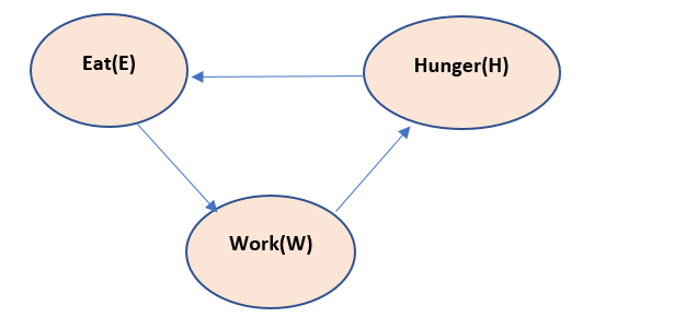
The above model reads like, if we work, we feel hunger. If we feel hunger – we eat. If we eat, we have energy to work.
Now this above model has a cycle in it and thus if chain rule is applied to it, the chain will become infinitely long. So, the above Bayesian model is not correct. Thus, we need to introduce the Latent variable here, let us call it as T
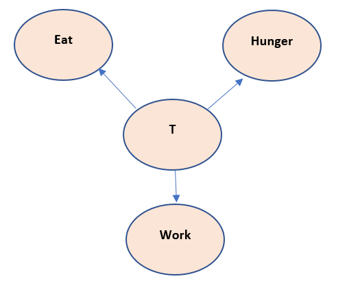
Now the above mode states that, T is responsible for eat, hunger and work to happen. This variable T is not observed but can be inferred as the cause of happening of work, eat and hunger. This assumption seems to be correct also, as in a biological body – something resides in it that pushes it to eat and work, even though we cannot observe it physically.
Let us write the chain rule equation for the above model:
P(W,E,H,T) = P(W/T)*P(E/T)*P(H/T)*P(T)
Another Example
Let us see another example. Suppose we have following variables: GPA, IQ, School. The model reads like if a person has good IQ, he/she will get good School and GPA, if he/she got good School, he/she will have good IQ and may get good GPA. If he/she gets good GPA, he/she may have good IQ, and he/she may be from good School. The model looks like:
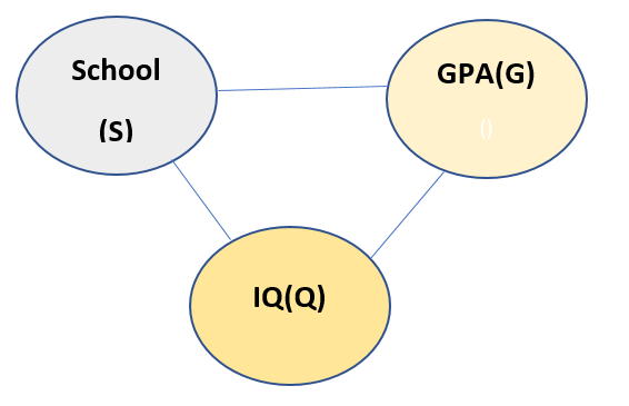
Now from above description of the model, all the nodes are connected to every other node. Thus chain rule cannot be applied to this model. So we need a Latent variable to be introduced here. Let us call the new Latent variable as I. The new model looks like:
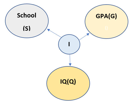
Now we read the above model as Latent variable I is responsible for all the other three variables. Now the chain rule can easily be applied. And it looks like:
P(S,G,Q,I) = P(S/I)*P(G/I)*P(Q/I)*P(I)
Hence in this post we saw how to model and create Latent Variables. They mostly help in reducing the complexity of the problem.
Now from then next post we will start much interesting part of Bayesian inferencing using the above Latent variables wherever required.
Thanks for reading!!!