
Last week, I gave a one-hour seminar covering one of the machine learning tools which I have used extensively in my research: neural networks. Preparation of the seminar was very useful for me since it required me to make sure that I really understood how the networks function, and I (think I) finally got my head around back-propagation — more on that later. In this post, and depending on length, the next (few), I intend to reinterpret my seminar into something which might be of use to you, dear reader. Here goes!
A neural network is a method in the field of machine learning. This field aims to build predictive models to help solve complex tasks by exposing a flexible system to a large amount of data. The system is then allowed to learn by itself how to best form its predictions.
An example of such a problem is shown below in which a neural network is tasked to predict the colour of points in 2-D space according to their positions.
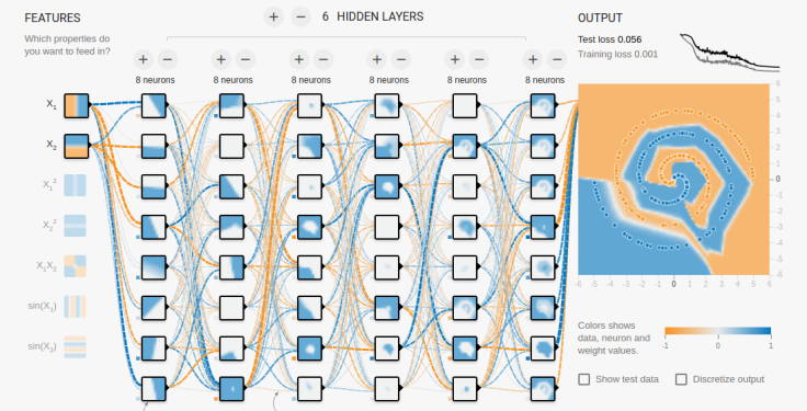
From the picture above, we can see that a neural network consists of three components: the inputs, features in the data; the network, layers of neurons; and the output, the prediction of the trained model. Additionally a method of the training the network is required, in order to make its predictions useful.
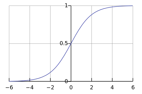
The fundamental component of a neural network is the neuron. Quite simply, this applies a mathematical function to inputs and passes the result on to other neurons. Each input into the neuron is weighted, and these weights are free parameters to be adjusted during training. The mathematical function is referred to as the activation function. Within the field of ML there are several common choices for the activation function (more on these later), but in principle anything which is continuously differentiable is applicable. An example might be the (in)famous sigmoid function:

The network is then many layers of neurons stacked together and connected up; the outputs of one layer are used as inputs to the next. By stacking layers together, the basic activation functions may be used to form more complex mathematical functions. The aim is to be able to build a function which maps the inputs to the desired outputs, as seen in the picture above where the output is simply a complex function of the two inputs.
Since the activation function of each neuron is (normally) the same, this complex function must be built by adjusting the weights each neuron applies to its inputs. One way to do this might be to test random settings for the weights, but this is unlikely to be effective for anything but tiny networks. Instead we some way to intelligently train the network. In order to do this, we first need to be able to quantify the performance of the network.
We refer to this as the loss function. Essentially it measures the difference between the network’s predictions for a set of training data, and what the outputs should have been (the true values). One common choice is the mean-squared-error:

This takes the average over a set of data of the squared difference between the predicted and true values for each data point. There are several other ways of defining the loss function, and the choice of which to use depends on the type of problem being solved. For instance, in classification problems, using the cross-entropy normally provides better results.
Now that we have a way of quantifying the current performance of our network, training it simply becomes an optimization problem of minimizing the loss function. The field of function optimization is pretty advanced, with methods like simulated annealing and genetic algorithms being able to find the global minima of black-box functions. However, because the of the huge number of free parameters (perhaps in the region O(10⁴)-O(10⁶)), these approaches are very slow to converge.
Luckily, whilst the loss function contains many local minima, the very things the advance algorithms are designed to deal with, each minima is about as optimal as any other. Effectively we just need to find the centre of a high-dimensional bowl, and for this the humble gradient-descent algorithm is perfect.
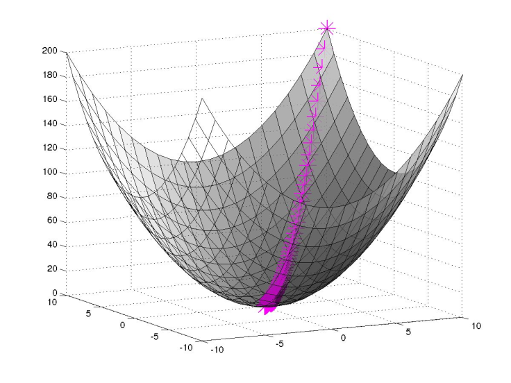
As its name suggests, the gradient-descent algorithm involves calculating the slope of the loss function at a given set of parameters and moving in the direction in which it is steepest. Evaluating the gradient can still be an expensive task, but for neural networks, there is a trick we make use of, and this will be the subject of my next post.