
In the previous article, we have tried to model the gold price in Turkey per gram. We will continue to do that to find the best fit for our data. When we chose the KNN and Arima model, we saw the traditional Arima model was much better than the KNN, which is a machine learning algorithm. This time we will try the regression model as a machine learning model and also try to improve our Arima model with some mathematical operations.
A regression that has Fourier terms is called dynamic harmonic regression. This harmonic structure is built of the successive Fourier terms that consist of sine and cosine terms to form a periodic function. These terms could catch seasonal patterns delicately.
}") ,
, }") ,
, }") ,
,
}") ,
, }") ,
, }") …
…
m is for the seasonal periods. If the number of terms increases, the period would converge to a square wave. While Fourier terms capture the seasonal pattern, the ARIMA model process the error term to determine the other dynamics like prediction intervals.
We will examine the regression models with K values from 1 to 6 and plot them down to compare corrected Akaike’s information criterion(AICc) measurement, which should be minimum. We will set the seasonal parameter to FALSE; because of that Fourier terms will catch the seasonality, we don’t want that the auto.arima function to search for seasonal patterns, and waste time. We should also talk about the transformation concept to understand the lambda parameter we are going to use in the models.
Transformation, just like differentiation, is a mathematical operation that simplifies the model and thus increases the prediction accuracy. In order to do that it stabilizes the variance so that makes the pattern more consistent. These transformations can be automatically made by the auto.arima function based on the optimum value of the lambda parameter that belongs to the Box-Cox transformations which are shown below, if the lambda parameter set to “auto“.
") ; if
; if 
 ; if otherwise
#Comparing with plotsplots <- list()for (i in seq(6)) { fit <- train %>% auto.arima(xreg = fourier(train, K = i), seasonal = FALSE, lambda = "auto") plots[[i]] <- autoplot(forecast(fit, xreg=fourier(train, K=i, h=18))) + xlab(paste("K=",i," AICC=",round(fit[["aicc"]],2))) + ylab("") + theme_light()}
gridExtra::grid.arrange( plots[[1]],plots[[2]],plots[[3]], plots[[4]],plots[[5]],plots[[6]], nrow=3)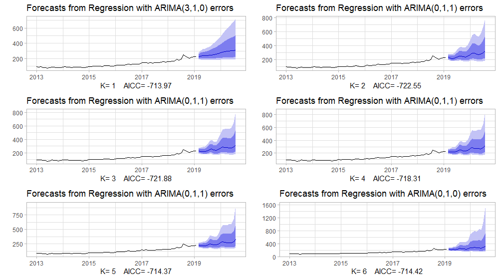
#Modeling with Fourier Regressionfit_fourier <- train %>% auto.arima(xreg = fourier(train,K=2), seasonal = FALSE, lambda = "auto")#Accuracyf_fourier<- fit_fourier %>%forecast(xreg=fourier(train,K=2,h=18)) %>%accuracy(test)f_fourier[,c("RMSE","MAPE")]# RMSE MAPE#Training set 8.586783 4.045067#Test set 74.129452 17.068118#Accuracy plot of the Fourier Regressionfit_fourier %>% forecast(xreg=fourier(train,K=2,h=18)) %>% autoplot() + autolayer(test) + theme_light() + ylab("")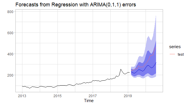 In the previous article, we have calculated AICC values for non- seasonal ARIMA. The reason we choose the non-seasonal process was that our data had a very weak seasonal pattern, but the pairs of Fourier terms have caught this weak pattern very subtly. We can see from the above results that the Fourier regression is much better than the non-seasonal ARIMA for RMSE and MAPE accuracy measurements of the test set.
Since we are also taking into account the seasonal pattern even if it is weak, we should also examine the seasonal ARIMA process. This model is built by adding seasonal terms in the non-seasonal ARIMA model we mentioned before.

}") : non-seasonal part.
: non-seasonal part._m}") : seasonal part.
: seasonal part. : the number of observations before the next year starts; seasonal period.
 (1, 1, 1)_{12}}") model for monthly data, m=12. This process can be written as:
model for monthly data, m=12. This process can be written as:

#Modeling the Arima model with transformed datafit_arima<- train %>% auto.arima(stepwise = FALSE, approximation = FALSE, lambda = "auto")#Series: .#ARIMA(3,1,2) with drift#Box Cox transformation: lambda= -0.7378559#Coefficients:# ar1 ar2 ar3 ma1 ma2 drift# 0.8884 -0.8467 -0.1060 -1.1495 0.9597 3e-04#s.e. 0.2463 0.1557 0.1885 0.2685 0.2330 2e-04#sigma^2 estimated as 2.57e-06: log likelihood=368.02#AIC=-722.04 AICc=-720.32 BIC=-706.01 |
 =-0.7378559.
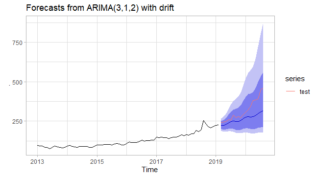
f_arima<- fit_arima %>% forecast(h =18) %>% accuracy(test)f_arima[,c("RMSE","MAPE")]# RMSE MAPE#Training set 9.045056 3.81892#Test set 67.794358 14.87034
The time-series data with weak seasonality like our data has been modeled with dynamic harmonic regression, but the accuracy results were worst than Arima models without seasonality.
In addition to that, the transformed data has been modeled with the Arima model more accurately than the one not transformed; because our data has the variance that has changed with the level of time series. Another important thing is that when we take a look at the accuracy plots of both the Arima model and Fourier regression, we can clearly see that as the forecast horizon increased, the prediction error increased with it.
The original article can be found here.
References
- Forecasting: Principles and Practice, Rob J Hyndman and George Athanasopoulos
- Statistic How To: Box-Cox Transformation
- Wikipedia: Fourier Series