
This article was written by Motoki Wu. Full title: How to construct prediction intervals for deep learning models using Edward and TensorFlow.
Edward and Tensorflow. Source: here (Duke University)
The difference between statistical modeling and machine learning gets blurry by the day. They both learn from data and predict an outcome. The main distinction seems to come from the existence of uncertainty estimates. Uncertainty estimates allow hypothesis testing, though usually at the expense of scalability.
Machine Learning = Statistical Modeling – Uncertainty + Data
Ideally, we mesh the best of both worlds by adding uncertainty to machine learning. Recent developments in variational inference (VI) and deep learning (DL) make this possible (also called Bayesian deep learning). What’s nice about VI is that it scales well with data size and fits nicely with DL frameworks that allow model composition and stochastic optimization.
An added benefit to adding uncertainty to models is that it promotes model-based machine learning. In machine learning, the results of the predictions are what you base your model on. If the results are not up to par, the strategy is to “throw data at the problem”, or “throw models at the problem”, until satisfactory. In model-based (or Bayesian) machine learning, you are forced to specify the probability distributions for the data and parameters. The idea is to explicitly specify the model first, and then check on the results (a distribution which is richer than a point estimate).
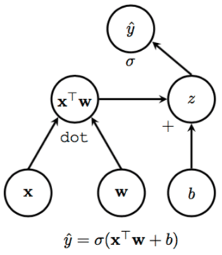
Bayesian Linear Regression
Here is an example adding uncertainty to a simple linear regression model. A simple linear regression predicts labels Y given data X with weights w.
Y = w * X
The goal is to find a value for unknown parameter w by minimizing a loss function.
(Y – w * X)²
Let’s flip this into a probability. If you assume that Y is a Gaussian distribution, the above is equivalent to maximizing the following data likelihood with respect to w:
p(Y | X, w)
So far this is traditional machine learning. To add uncertainty to your weight estimates and turn it into a Bayesian problem, it’s as simple as attaching a prior distribution to the original model.
p(Y | X, w) * p(w)
Notice this is equivalent to inverting the probability of the original machine learning problem via Bayes Rule:
p(w | X, Y) = p(Y | X, w) * p(w) / CONSTANT
The probability of the weights (w) given the data is what we need for uncertainty intervals. This is the posterior distribution of weight w.
Although adding a prior is simple conceptually, the computation is often intractible; namely, the CONSTANT is a big, bad integral.
Monte Carlo Integration
An approximation of the integral of a probability distribution is usually done by sampling. Sampling the distribution and averaging will get an approximation of the expected value (also called Monte Carlo integration). So let’s reformulate the integral problem into an expectation problem.
The CONSTANT above integrates out the weights from the joint distribution between the data and weights.
CONSTANT = ∫ p(x, w) dw
To reformulate it into an expectation, introduce another distribution, q, and take the expectation according to q.
∫ p(x, w) q(w) / q(w) dw = E[ p(x, w) / q(w) ]
We choose a q distribution so that it’s easy to sample from. Sample a bunch of w from q and take the sample mean to get the expectation.
E[ p(x, w) / q(w) ] ≈ sample mean[ p(x, w) / q(w) ]
This idea we’ll use later for variational inference.
Variational Inference
The idea of variational inference is that you can introduce a variational distribution, q, with variational parameters, v, and turn it into an optimization problem. The distribution q will approximate the posterior.
q(w | v) ≈ p(w | X, Y)
These two distributions need to be close, a natural approach would minimize the difference between them. It’s common to use the Kullback-Leibler divergence (KL divergence) as a difference (or variational) function.
KL[q || p] = E[ log (q / p) ]
The KL divergence can be decomposed to the data distribution and the evidence lower bound (ELBO).
KL[q || p] = CONSTANT – ELBO
The CONSTANT can be ignored it since it’s not dependent on q. Intuitively, the denominators of q and p cancel out and you’re left with the ELBO. Now we only need to optimize over the ELBO.
The ELBO is just the original model with the variational distribution.
ELBO = E[ log p(Y | X, w)*p(w) – log q(w | v) ]
To obtain the expectation over q, Monte Carlo integration is used (sample and take the mean).
In deep learning, it’s common to use stochastic optimization to estimate the weights. For each minibatch, we take the average of the loss function to obtain the stochastic estimate of the gradient. Similarly, any DL framework that has automatic differentiation can estimate the ELBO as the loss function. The only difference is you sample from q and the average will be a good estimate of the expectation and then the gradient.
To read the rest of the article with source code and computation of prediction intervals, click here.