
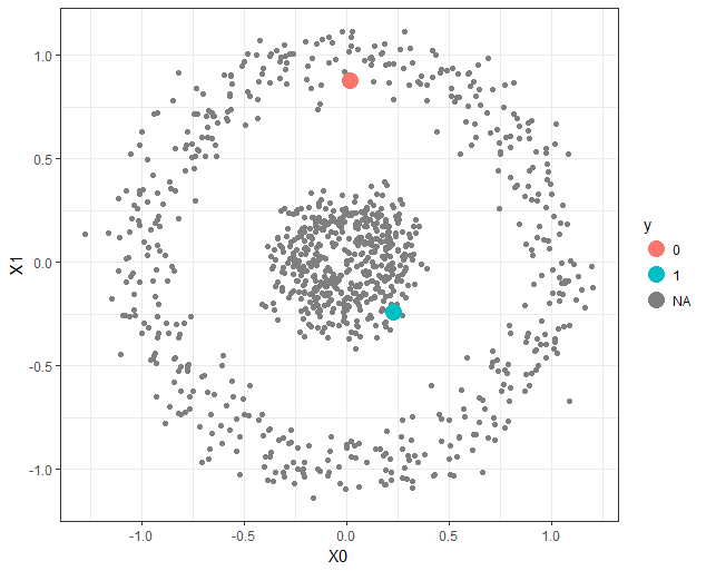
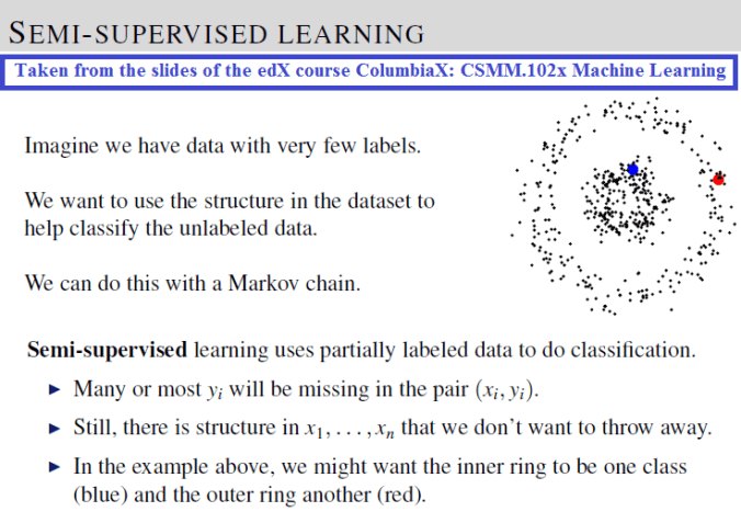
In this article, a semi-supervised classification algorithm implementation will be described using Markov Chains and Random Walks. We have the following 2D circles dataset (with 1000 points) with only 2 points labeled (as shown in the figure, colored red and blue respectively, for all others the labels are unknown, indicated by the color black).
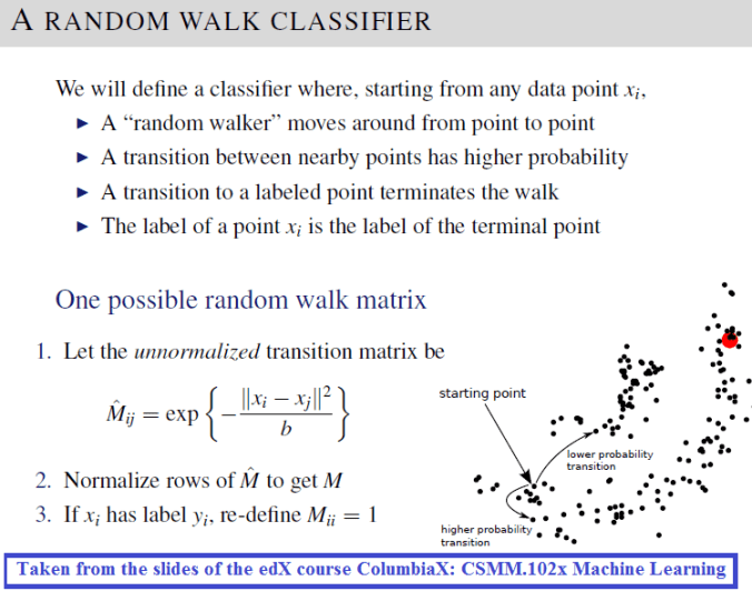
Now the task is to predict the labels of the other (unlabeled) points. From each of the unlabeled points (Markov states) a random walk with Markov transition matrix (computed from the row-stochastic kernelized distance matrix) will be started that will end in one labeled state, which will be an absorbing state in the Markov Chain.
This problem was discussed as an application of Markov Chain in a lecture from the edX course ColumbiaX: CSMM.102x Machine Learning. The following theory is taken straightway from the slides of the same course:
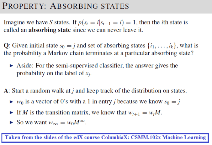
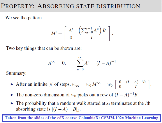
Since here the Markov chain does not satisfy the connectedness condition of the Perron-Frobenius theorem, it will not have a single stationary distribution, instead for each of the unlabeled points the random walk will end in exactly one of the terminal (absorbing) state and we can directly compute (using the above formula, or use power-iteration method for convergence, which will be used in this implementation) the probability on which absorbing state it’s more likely to terminate starting from any unlabeled point and accordingly label the point with the class of the most probableabsorbing state in the Markov Chain.
The following animation shows how the power-iteration algorithm (which is run upto 100 iterations) converges to an absorbing state for a given unlabeled point and it gets labeled correctly. The bandwidth b for the Gaussian Kernel used is taken to be 0.01.
As can be seen, with increasing iterations, the probability that the state ends in that particular red absorbing state with state index 323 increases, the length of a bar in the second barplot represents the probability after an iteration and the color represents two absorbing and the other unlabeled states, where the w vector shown contains 1000 states, since the number of datapoints=1000.
Now, for each of the unlabeled datapoints, 500 iterations of the power-iteration algorithm will be used to obtain the convergence to one of the absorbing states, as shown. Each time a new unlabeled (black) point is selected, a random walk is started with the underlying Markov transition matrix and the power-iteration is continued until it terminates to one of the absorbing states with high probability. Since only two absorbing states are there, finally the point will be labeled with the label (red or blue) of the absorbing state where the random walk is likely to terminate with higher probability. The bandwidth b for the Gaussian Kernel used is taken to be 0.01. Off course the result varies with kernel bandwidth. The next animation shows how the unlabeled points are sequentially labeled with the algorithm.