
The work of an Italian mathematician in the 1930s may hold the key to epidemic modeling.
That’s because models that try to replicate reality in all its detail have proven hard to steer during this crisis, leading to poor predictions despite noble and urgent efforts to recalibrate them. On the other hand overly stylized compartmental models have run headlong into paradoxes such as Sweden’s herd immunity.
A theorem of de Finetti inspires a different approach.
- We identify orbits in the space of models (to be explained) that leave unchanged the key decision making quantities we care about.
- We use mixtures of IID models to span the orbits, assisted by convexity calculations.
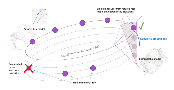
This approach is represented in the picture above. The important thing to note is that we are not attempting to find a model that is close to the truth, only close to the orbit. This will make a lot more sense after Section 1, I promise.
Outline
- An introduction to de Finetti’s Theorem
- Nature’s model for an epidemic … somewhere in a large space
- Most important questions are symmetrical
- The orbit of the symmetric group
- Finding the orbit
1. Introducing de Finetti’s Theorem … or something close to it
Two nearby hospitals risk running out of supplies. Joe and Mary are engaged to build a probabilistic model for binary outcomes. Either there will be a shortage or not. Four possible outcomes in total. Mayor Pete lays out the rules, also noting that only coins may be deployed for this particular stochastic modeling exercise.
- Both locations should have 50% chance of a shortage
- Outcomes must be positively correlated
- The hospitals are interchangeable
Joe is the first to return. He explains that his model uses conditional probability to link the fates of the two hospitals. He flips one coin to determine the fate of hospital A. Then (the part that took him longer to figure out) he flips more coins and begins recording the sequence until either HTH or TTH appears. The former will happen first with 3/8 probability, he explains, in which case he assigns an outcome to hospital B that is the opposite of hospital A’s outcome. Otherwise, with 5/8 probability, it will be the same. Joe is beaming with pride.
Mary goes next. Well, she says, it is obvious that I can use two coins to generate a 1 in 4 chance of a shortage. So I just do that twice, once for each hospital.
Mayor Pete looks at Mary aghast. Not only has Mary failed to link the fates of the two hospitals, she apparently has ignored his first rule entirely. Well at least you used coins, he says. But did I not tell you that each hospital has a fifty fifty chance? Oh yes, says Mary. I know. I reverse the result every other time.
Right says Mayor Pete, rolling his eyes, I’m going to use Joe’s model. But Mary, if you don’t mind I’d like to use yours as a backup. Mary graciously agrees and for the next several days supplies Mayor Pete with calculations that he requests, all of which are based on the probabilities of the four outcomes. Mayor Pete requires insurance calculations, risk measures and various metrics to guide decision making.
The next week Mayor Pete summons Joe and Mary to his office. To their mutual surprise he launches into an accusation of collusion, throwing Joe and Mary’s results back at them and demanding to know why they are identical in every respect. Do you not realize how important this is, he asks? There is a reason I want a second opinion. Joe is stunned, but Mary casually takes out a pen and demonstrates wordlessly how many times on average each model will produce each of the four outcomes, given 32 chances to do so.

It seems Mary knew what she was doing after all. Her approach has another advantage that will be important to us. The joint probabilities in Joe’s model (i.e. 6/32 and 10/32) cannot be written as a product of individual probabilities of hospital outcomes. But on Mary’s side of the equation, notice that this is possible for each of the two matrices individually.
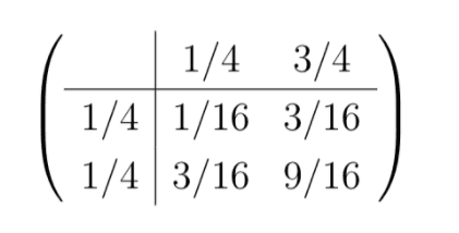
She has demonstrated that Joe’s model, in which hospital outcomes are explicitly connected, is equivalent to a mixture of two models in which the hospitals are independent. Moreover we also notice that in each of the scenarios that comprise Mary’s mixture, the probabilities of outcomes are the same for hospital A and hospital B. The hospitals are not only independent but also identically distributed.
This can be viewed as a finite dimensional rendering of the celebrated theorem of Bruno de Finetti. That theorem says that any model for exchangeable random variables can be decomposed into a mixture of much simpler models in which variables are independent and identically distributed. Joe can try to be creative, but assuming strong correlation between hospitals Mary’s approach may be a more straightforward path.
The implications of de Finetti’s Theorem, both practical and philosophical, are quite far reaching. The theorem is sometimes used to motivate Bayesian statistics. It has been called the fundamental theorem of statistical inference. Certainly if one is faced with the need to produce an exchangeable model for something it should come to mind. More pertinently for us, it may be informative when one is faced with a mathematical conundrum that seemingly remains the very same conundrum after some rearranging of deck chairs.
2. Nature’s model for an epidemic may be subtle
Before we get to that, let’s agree on a vast space of possible models that might encompass the true one. We shall assume the following of an epidemic:
- The world is divided into M regions that don’t interact
- Within each region are N neighborhoods that do interact
These are the only assumptions, so we have done little to tie nature down. We suggest that there is one true model for a region. It gets played out M times with different results each time. Nature’s model is extremely complicated, no doubt, but despite the hint I have given regarding de Finetti’s Theorem, there is no requirement that neighborhoods are treated equally. One neighborhood’s odds may be skewed more than another’s. The joint distribution of the trajectories of neighborhoods may be well beyond our modeling abilities despite all the tools of stochastic modeling at our disposal.
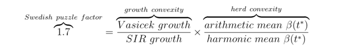
As we are learning, nature may play a stranger game of chess than we imagined. In a previous article I considered the curious relationship between herd immunity and early stage growth. The space of models probably includes an orbit where this happens:
- Observation #1: In the early stages, doubling times are under a week
- Observation #2: Peak infection occurs at 20% penetration.
The classic SIR epidemiological model is an example of an approach that refuses to bend to this kind of observation and instead, snaps in two. We quickly review that failure played backwards from #2 to #1.
- Observation #1 means that the actual number of people being infected every day, relative to the number of people who are contagious, must be 4/5th’s of what it started out as (the susceptible population has dropped to 80%, so the chance of running into someone you can infect has dropped by a factor of 0.8). So if things are balanced, it must be that infection was 5/4th’s of recovery back when the susceptible population was close to 100%.
- The difference between 5/4 and 1 is 1/4. That excess infection versus recovery translates to 25% growth, when measured in units of the typical generation time which we shall assume is 7.5 days. Our doubling time is 23 days, much larger than a week as demanded by Observation #1.
Thus it seems like a very bad idea to assume nature falls within that particular class of models, and better to work back from extremely mild assumptions about what is true. I have assumed only one shortcoming of nature’s model – regions are independent. Of course we know that regions will interact, in reality, that would seem to be the definition of a pandemic. But neighborhoods are likely to interact a lot more and so this is perhaps a simplification we might live with. You might even try to remove it by assuming the global dependence is driven by one factor.
3. Most questions are symmetrical
The following are important for decision making:
- A count of the number of cases at a given time
- The time of peak infection
- The slope of the time series of cases on a logarithmic plot
- Doubling times
- Estimates of total use of ICU units extrapolated from the model
And we could list many more. These are aggregate statistics. They are left unchanged if we swap the roles of neighborhoods at the start of the simulation. I won’t belabor this point because it is obvious, but when combined with de Finetti’s Theorem it goes a long way.
4. The orbit of the symmetric group
Our hunt for nature’s true model will never succeed, at least in this particular post. However we will try to locate a symmetrized version of that model. This is nature’s model shuffled. We explain the symmetrizing operation using something that is easier to visualize.
Permuting a model for three dice
Let’s start with dice. For this purpose, let us suppose Model A assigns probabilities to the outcomes of three dice. For convenience Die1=X, Die 2=Y and Die 3=Z and outcomes are labeled x, y and z. Model B is very similar to Model A. The models assign probabilities as follows:
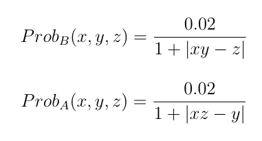
where the 0.02 is approximate. Not quite the same, but obviously similar. Both models assign higher probabilities to combinations of die rolls when the product of two dice is close to the third. However as we move from Model A to Model B we exchange the roles of the dice. Because this is the only change, we say that Model A and Model B lie in the same orbit of the symmetric group, which is the set of all permutations of models. Each model may be viewed as permuting the inputs of the others (as we all can do by accident when passing positional arguments to functions in the wrong order).
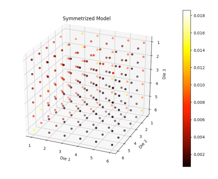
Here we show the probabilities of all three die outcomes for Model A. Different colors correspond to different probabilities.
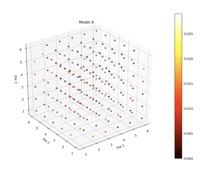
The most likely outcome is (1,1,1). There is a lot going on in this picture (normal dice would of course show all dots the same color). Here’s a home-buyers walkthrough of Model B’s living room:
Symmetrizing a model for three dice
There is a similar model for the three dice that treats each die on an equal footing.
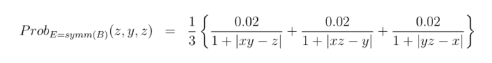
The E stands for “Exchangeable”. Notice that if you take any re-ordering of x, y and z this probability is left unchanged. However there is still plenty of structure in the model as you can see from the probabilities it assigns to each of the 216 possible outcomes.
In our case the exchangeable model E and the non-symmetric models A and B all lie on the same orbit. To create the symmetrized model I took an average of three models that were similar to A and B but permutations of each other. In general if we have a model for n variables the symmetrizing operator acting on a model might be written
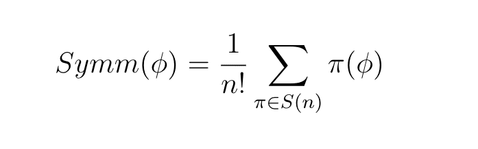
where the average is over all possible rule changes where we interchange the roles of variables. Notice this is an average over the orbit. There are six permutations of three objects but we only needed three due to symmetry in the formula.
Now suppose I have some quantity of interest I want to compute that is symmetric itself. For example we might be interested in the probability that the product of three dice exceeds 10. The answer we get will be exactly the same for all three models, and for that matter any model on the same orbit. Thus…
Any model on nature’s orbit will do
Moving from dice back to models for epidemics in neighborhoods, and taking as a given that many if not most important questions are symmetric, we realize that any model on the same orbit is as good as another. For example, suppose we are interested in the number of infections after three days. We have
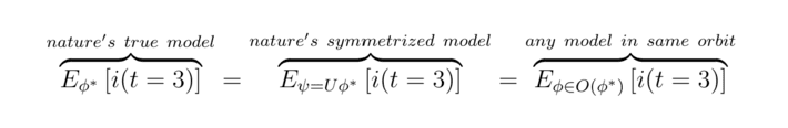
thus we will accidentally get the right answer, as it were, so long as we are close to the orbit.
5. Finding the orbit
We can find the right orbit using IID models and convexity adjustments.
De Finetti’s theorem suggests a mixture of IID models might be near the orbit
Based on the experience of Joe and Mary we make one final supposition. Not only can we pick any model on the orbit, but there is a good chance that a mixture of independent identically distributed models may get us there. In the dice picture this means that we’d consider mixtures of models that treat each die as an independent roll. In the case of our epidemic model it would mean that each neighborhood does not interact with the others.
Of course assuming no interaction is not a good assumption in isolation, but by taking different mixtures of these models we create dependence. And we will generate a whole bunch of exchangeable models. We know that there is an exchangeable model on every orbit because you can apply the symmetrization operations, and a little reflection might convince you there is exactly one. So as we change up the mixture we will be rapidly traversing the orbits, visiting a lot of exchangeable models and maybe even all of them. Whereas if we were just tinkering with a model that has 10,000 lines of code and exists in the very high dimensional space of models, we might be making a lot of sideways movement.
Here’s an attempt at a “big picture”:
It is certainly big. Can we justify it?
- No matter how complex nature’s model is, there is a symmetrical equivalent.
- The exchangeable model provides the same answers (to symmetrical questions)
- The exchangeable model is a mixture of simple IID models (de Finetti’s Theorem)
It doesn’t matter that we will never get our hands on the truth, which we won’t. It also doesn’t matter that we wouldn’t be able to physically implement the symmetrization operator that moves natures’ model around the orbit to its exchangeable representative. We don’t have to (which is good because by the time you get to 60 neighborhoods that is one permutation for every electron in the universe).
Point 2 is intuitively obvious I hope. (Physicists: You might like to think of this as moving an operator from the “bra” to the “ket”, and you can define the action of permutation on functions in a contragredient fashion if you wish).
Point 3 is de Finetti’s Theorem, in spirit. It is only technically true if we allow signed probabilities but as a practical matter it is probably good enough with unsigned. It says we can use independent identically distributed (iid) models for neighborhoods – which means that we only need a model for one neighborhood and we assume they all evolve independently. This decomposition is rather remarkable but Mary has prepared us for the surprise.
Do we need negative weights in the mixture?
It is possible that nature has chosen a model which cannot be decomposed into a positive weighted combination of iid models. Then again, this might not be the end of the world. We can allow a few small negative weights in the mix even if this feels a little strange (given that the weight we assign to our simple models is interpreted as a probability). Better people like Feynman and Dirac found negative probabilities on the route to useful numbers.
“Negative energies and probabilities should not be considered as nonsense. They are well-defined concepts mathematically, like a negative of money” – Paul Dirac, 1942
Then there’s the Wigner quasiprobability distribution … for another day.
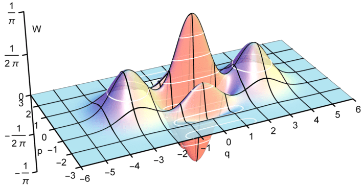
[ Wigner Quasiprobability Function courtesy of Geek3 ]
My point: panic isn’t a requirement should negative probabilities show up – though in fact they are less likely to show up in the first place because epidemics are a classic case of strong dependence (and this diminishes the need for minus signs). That’s why I claim it doesn’t matter terribly much that de Finetti’s original theorem applies to infinite sequences of neighborhoods rather than finite collections, though this part of my argument could benefit from generalizations of de Finetti’s Theorem I am sure.
A few years ago I had the pleasure of working with Gabor Szekely who proved a number of results about the finite case. Not being as clever as him my comments are based more on numerical experiments. There are some links to other articles on the finite case below.
Mixing deterministic disease models
Now there is another strong reason to use simple mixtures of independent identically distributed models – it is very easy to compute things. For instance:
- The model for each neighborhood is a classic epidemiological model like SIR
- We take a mixture of them
We don’t have to believe the neighborhoods are really independent because the mixing takes care of that. Now to fit to observed phenomena we can:
- Use existing results for model predictions
- Compute convexity adjustments that take account of the mixing
- Invert the convexity adjustment to find the right orbit
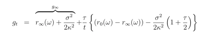
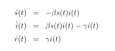
To proceed, the constant parameter SIR model is:
Now allow beta to be varied in the de Finetti mixture according to some variation function
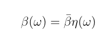
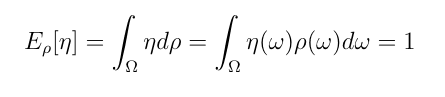
where eta has unit norm with respect to population density rho
Then in our mixture model at herd immunity the number of susceptible people is
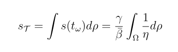
This is the usual answer divided by the harmonic mean of eta. The harmonic mean is known in closed form for a number of distributions which you can see from the Wikipedia page for harmonic mean. You can invert these formulas to correct for how far wrong the standard model is and you’ll get much closer to the orbit of nature’s model.
A word of warning here that you really want to average cases where beta exceeds gamma only, so it is close to a harmonic mean but not exactly the same.
Mixing stochastic models
I think a better approach than mixing deterministic models, and more true to de Finetti’s theorem, is to use a mixture of stochastic disease models. Here I would suggest browsing the Fixed Income Modeling section of the library and not just Epidemiology.
The terms on the right hand side have closed form formulas, or good approximations, so backing into the right amount of variation is in principle easy.
Takeaway
When epidemic models are chosen at the level of equivalence classes under permutation, which is to say picking an orbit of the symmetric group, it is difficult to go wildly wrong and also much harder to waste effort moving around an orbit (rather than up and down to traverse all the exchangeable models). Aided by convexity adjustments, mixtures of independent identically distributed models are very easy to use and the work of de Finetti and others has taught us about their span. The strong dependence between outcomes suggests to me that de Finetti’s Theorem is indeed fundamental to epidemic modeling.
Of course de Finetti’s Theorem is already pretty fundamental to statistics, if not quite rising to the status of “the” fundamental theorem because there isn’t one. As an aside we have a Fundamental Theorem of Algebra, a Fundamental Theorem of Arithmetic, a Fundamental Theorem of Calculus and a Fundamental Theorem of Linear Algebra but no Fundamental Theorem of Statistics. A frontrunner must be the Central Limit Theorem (which is, after all the Central Limit Theorem and not the Central Limit Theorem – something I only recently learned) but perhaps I have convinced you that de Finetti’s Theorem is another strong candidate.
If not, perhaps there is an opening in Epidemiology.
Related posts
On the topic of convexity adjustments to help find the right orbit:
- Reconciling herd immunity and growth with the Vasicek model
- Infection attenuation due to repeated contact
- Herd immunity and the harmonic mean
- A way to add even more variation (regime switching Vasicek)
Readings related to de Finetti’s Theorem (finite case)
- Finite exchangeable sequences, Diaconis and Freedman
- de Finetti’s Theorem for Abstract Finite Exchangeable Sequences, Kerns and Szekely (paywalled)
- Alternative approach by Janson, Konstantopoulos and Yuan
Originally posted here