
With explainable AI, intuitive parameters easy to fine-tune, versatile, robust, fast to train, without any library other than Numpy. In short, you have full control over all components, allowing for deep customization, and much fewer parameters than in standard architectures.
Introduction
I explore deep neural networks (DNNs) starting from the foundations, introducing a new type of architecture, as much different from machine learning than it is from traditional AI. The original adaptive loss function introduced here for the first time, leads to spectacular performance improvements via a mechanism called equalization.
To accurately approximate any response, rather than connecting neurons with linear combinations and activation between layers, I use non-linear functions without activation, reducing the number of parameters, leading to explainability, easier fine tune, and faster training. The adaptive equalizer – a dynamical subsystem of its own – eliminates the linear part of the model, focusing on higher order interactions to accelerate convergence.
One example involves the Riemann zeta function. I exploit its well-known universality property to approximate any response. My system also handles singularities to deal with rare events or fraud detection. The loss function can be nowhere differentiable such as a Brownian motion. Many of the new discoveries are applicable to standard DNNs. Built from scratch, the Python code does not rely on any library other than Numpy. In particular, I do not use PyTorch, TensorFlow or Keras.
10 Key Features to Boost DNN Performance
Here is a high-level summary of key features that boost performance, in simple English. Most apply to any deep neural network. Also, the focus is on the core engine that powers all DNNs: gradient descent, layering and loss function.
- Reparameterization — Typically, in DNNs, many different parameter sets lead to the same optimum: loss minimization. DNN models are non-identifiable. This redundancy is a strength that increases the odds of landing on a good solution. You can change the parameterization to reduce redundancy and increase identifiability. You achieve this by reparameterization and eliminating intermediate layers. It usually does not improve the results. Or you can do the opposite: add redundant layers to increase leeway. Or you can transform parameters while keeping them in the same range. For instance, use θ’ = θ2 instead of θ, both in [0, 1]. This flexibility allows you to achieve better results but require testing.
- Ghost parameters — Adding artificial, non-necessary or redundant parameters can make the descent more fluid. It gives more chances (more potential paths) for the gradient descent to end in a good configuration. You may use some of these ghost parameters for watermarking your DNN, to protect your model against hijacking and unauthorized use.
- Layer flattening — Instead of hierarchical layers, you can optimize the entire structure at once, across all layers. That is, minimizing the loss function globally at each epoch rather than propagating changes back and forth throughout many layers. It reduces error propagation and eliminates the need for explicit activation functions. It may reduce the risk of getting stuck (gradient vanishing).
- Sub-layers — In some sense, it is the oppositive of layer flattening. At each epoch, you minimize the loss iteratively, for a subset of parameters (sub-layer) at a time, keeping the other parameters unchanged. It works as in the EM algorithm. Each parameter subset optimization is a sub-epoch within an epoch. A full epoch consists of going through the full set of parameters. This technique is useful in high dimensional problems with complex, high-redundancy parameter structure.
- Swarm optimization — Handy for lower dimensional problems with singularities and non-differentiable loss function. You start with multiple random initial configurations (called particles) in the gradient descent. For each particle, you explore random neighbors in the parameter space and move towards the neighbor that minimizes the loss. You need a good normalization of the learning rate to make it work. Consider working with adaptive learning rates that depend on the epoch and/or axis (different learning rate for each axis, that is, for each parameter).
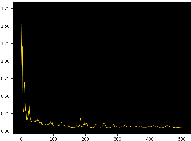
- Decaying entropy — Instead of descending all the time, allow for occasional random ascents in the gradient descent. Globally or for specific parameters chosen randomly. Especially in the earlier epochs. Think of it like a cave exploration: to reach the very bottom of a deep cave, sometimes you need to go up through a siphon and climb back up from it on the other side to be able to further go down. Otherwise, you get stuck in the siphon. The hyperparameter controlling the ups and downs is the temperature. At zero, the descent is a pure descent with no ups. I call it chaotic gradient descent as it is different from stochastic descent. See Figure 2.
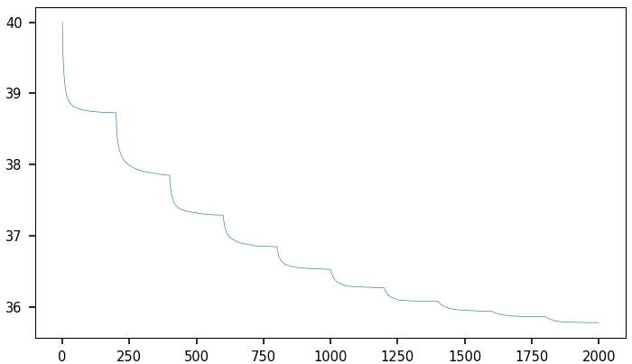
- Adaptive loss — Some knobs turn the loss function into one that changes over time. In one case, I force the loss function to converge towards the model evaluation metric via a number of transitions over time. These changes in the loss function typically take place when the gradient descent stops improving, re-accelerating the descent to move away from a local minimum. See Figure 1.
- Equalization — In my implementation, this is the feature that led to the biggest improvement: reducing the number of epochs thus accelerating convergence along with eliminating a number of gradient descent issues. It consists of replacing the fixed response y at each epoch by an adaptive response y’ = φ(y, α). Here φ belongs to a parametric family of transforms indexed by α, and stable under composition and inversion. For instance, scale-location transforms. So, even if you don’t know the history of the successive transforms with a different data-driven α at each epoch, it is very easy at the end to apply an inverse transform to map the final response back to its original, via ordinary least squares. You apply the same inverse transform to predicted values.
- Normalized parameters — In my implementation all parameters are in [0, 1]. Also true for the input data after normalization. To use parameters outside that range, use reparameterization, for instance θ’ = 1 / (1 – θ) while optimizing for θ in [0, 1]. This approach eliminates gradient explosion.
- Math-free gradient — No need to use chain rules and other math formula to compute the partial derivatives in the gradient. Indeed, you don’t even need to know the mathematical expression of the loss function. It works on pure data without math functions. Numerical precision is critical. Some math functions are pre-computed in 0.0001 increments and stored as a table. This is possible because the argument (a parameter) is in [0, 1]. It can significantly increase speed.
Parameters in my model have an intuitive interpretation, such as centers and skewness, corresponding to kernels in high-dimensional adaptive kernel density estimation or mixtures of Gaussians that can model any type of response. In some cases, the unknown (predicted) centers are expected and visible in the response such as in clustering problems. Sometimes — depending on the settings — they are not and act as hidden or latent parameters.
Finally, while I implicitly use tensors, you don’t need to know what a tensor is and there is no call to libraries such as TensorFlow.
Get the Full Code and Documentation
The PDF with many illustrations is available as paper 55, here. It also features the Python code (with link to GitHub), the replicable data generated by the code, the theory, and various options including for evaluation. The blue links in the PDF are clickable once you download the document from GitHub and view it in any browser. Keywords highlighted in orange are index keywords.
Conclusions
This original non-standard DNN architecture turns black boxes into explainable AI with intuitive parameters. The focus is on speed (fewer parameters, faster convergence), robustness, and versatility with easy, rapid fine-tune and many options. It does not use PyTorch or similar libraries: you have full control over the code, increasing security and customization. Tested on synthetic data batches for predictive analytics, high dimensional curve fitting and noise filtering in various settings, it incorporates many innovative features. Some of them, like the equalizer, have a dramatic impact on performance and can also be implemented in standard DNNs. The core of the code is simple and consists of fewer than 200 lines, relying on Numpy alone.
About the Author

Vincent Granville is a pioneering GenAI scientist, co-founder at BondingAI.io, the LLM 2.0 platform for hallucination-free, secure, in-house, lightning-fast Enterprise AI at scale with zero weight and no GPU. He is also author (Elsevier, Wiley), publisher, and successful entrepreneur with multi-million-dollar exit. Vincent’s past corporate experience includes Visa, Wells Fargo, eBay, NBC, Microsoft, and CNET. He completed a post-doc in computational statistics at University of Cambridge.