
[Introduction of Association Rules]
Sometimes, the anecdotal story helps you understand the new concept. But, this story is real. About 15 years ago, in Walmart, a sales guy made efforts to boost sales in his store. His idea was simple. He bundled the products together and applied some discounts to the bundled products. (Now, it became common practices in marketing) For example, this guy bundled bread with jam, so that customers easily found them together. Moreover, customers could afford to buy them together as the bundled product was discounted. In this way, we can expect an increase in the revenue.
As bread and jam was so classical, so that he was determined to analyze all sales records in a hope of seizing new opportunities. He found interesting. Many many customers who bought diapers also purchased beers.


Seemingly, those are totally unrelated. He decided to dig deeper. He realized that it was arduous to raise kids (It doesn’t change at all in nowadays) So, the parents impulsively decided to purchase beer to relieve their stress. He bundled diapers and beers together. The sales skyrocketed. Still, this remains the perfect example of Association Rules in data mining. (Thank you professor Sun in University of Notre Dame! He gave this example in Business Intelligence class)
[About data]
Now, let’s suppose that you own Sephora, the largest cosmetic chain in United States (And probably in the world) You are selling 14 products in your store. Just like Walmart sales guy, you hope to boost your sales with the same technique. How do we go about doing this?
Your products: Brushes, Mascara, Eye shadow, Bronzer, Lip liner, Nail Polish, Lipstick, …
(To be honest, as a male, I have no idea what these products are)
Usually, sales data take on this form. It has a transaction number and corresponding items that our customers buy. Usually, when you extract the data from database(MS-SQL, Oracle whatever), it is supposed to be like this. First column is a transaction number, and second column is the item. So according to these data, our customer 1 purchased Blush, Bronzer, Brushes, Concealer, Eyeliner, Lip liner, Mascara, and Nail Polish at once. (I am not sure females purchased cosmetics in bulk actually)

However, in order to be used in R, it should take on this form. It doesn’t have any transaction number. You need to vertically arrange items that our customer purchased in a single transaction. I am going to offer you this data in the source code.

I’ll briefly touch on how to change the form of the data later.
[Terms that you should know]
You need to understand several key concepts regarding association rules.
1. A=>B
We call “A” as “LHS(Left-hand side),” and “B” as “RHS(Right-hand side)”
Let’s assume that A is diaper and B is beer. It means when a customer buys diaper, she would buy beer too.
2. Support
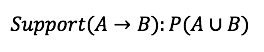
Let me get back to Walmart’s story. In this case, support means the probability of the customer buying diaper and beer together among all sales transactions.
3. Confidence

Suppose that if a customer pick up diaper. How he/she is likely to buy beer? The answer is “confidence” The maximum value of confidence has to be 1.
4. Lift

Lift is a true comparison between naive model and our model, meaning that how more likely a customer buy both, compared to buy separately? Lift 1 means, our customers are as likely to buy both diaper and beer together as buy them separately. Generally, in order to be meaningful in marketing, lift has to be greater than 1.
[Codes]
Unlike our theory, the code is simple. “arules” package allows you to do this really simply. just 4 lines. That’s all.
#Association Rule
library(arules)
myurl <- “https://docs.google.com/spreadsheets/d/18KBtFWkMq1Q9mOSVo9Q55GJ9IeC3NRYRn7yV5Id3z6A/pub?gid=0&single=true&output=csv”
data.raw <- read.transactions(url(myurl), sep=”,”) #Please use read.transactions! It’s not read.csv!
rules<-apriori(data.raw)
inspect(rules)
[Interpretation]
> inspect(rules)
lhs rhs support confidence lift 1 {Brushes} => {Nail Polish} 0.1556949 1.0000000 3.4178572 {Mascara} => {Eye shadow} 0.3354232 0.8991597 2.2585193 {Eye shadow} => {Mascara} 0.3354232 0.8425197 2.2585194 {Bronzer,Brushes} => {Nail Polish} 0.1013584 1.0000000 3.4178575 {Bronzer,Lip liner} => {Concealer} 0.1076280 0.8046875 1.742276
…
Well, this looks good. However, like I said, the higher lift is, the more it is meaningful in marketing sense. Let’s sort it from high lift to low lift, which allows us to identify strong correlation.
> rules.sorted <- sort(rules, by=”lift”)
> inspect(rules.sorted)
lhs rhs support confidence lift
1 {Brushes} => {Nail Polish} 0.1556949 1.0000000 3.417857
4 {Bronzer,Brushes} => {Nail Polish} 0.1013584 1.0000000 3.417857
26 {Blush,Concealer,Eye shadow} => {Mascara} 0.1243469 0.9596774 2.572581
18 {Blush,Eye shadow} => {Mascara} 0.1765935 0.9285714 2.489196
13 {Eye shadow,Nail Polish} => {Mascara} 0.1243469 0.9083969 2.435115
23 {Concealer,Eye shadow} => {Mascara} 0.1870428 0.8905473 2.387265
Let’s highlight the first row. Support is 0.1556, meaning that customers buy Brushes and Nail Polishes altogether by 15.56% among all transactions. Confidence is 100%, meaning that all brush buyers purchase nail polish (It’s huge!). Lift is 3.41, meaning that our customers are 3.41 times more likely to buy brushes and nail polish altogether than buy them separately!
In next section, we are going to prune the result.
More code? Click here!
)