Linear Regression Geometry

Linear Regression is one of the most widely used statistical models. If Y is a continuous variable i.e. can take decimal values, and is expected to have linear relation with X's variables, this relation could be modeled as linear regression, mostly the first model to fit,if we are planning to develop a model of forecasting Y or trying to build hypothesis about relation Xs on Y.

The general approch is to understand the theory based on principle of "minimum" square error and we derive the solution using minimization of functions through calculus,however it has a nice geometric intuition, if we use the tricks or methods related to solving an over-determined system

The objective of the linear regression is to express a dependent variable in terms of linear function of independent variables, if we have one independent variable, we can it simple (some call it uni-variate) linear regression or single variable linear regression and when we have many, we call it multiple linear regression, it is NOT multi-variate, the multi-variate linear regression refers to when we have more than one decedent variables.

1. Scatter Plot

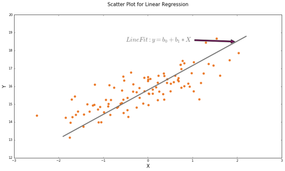
Without much of mathematics and symbols, the idea of linear regression could be explored through a scatter plot.We generate a sample of X and Y from normal distribution.

Linear Regression is about fitting a straight line from the scatter plot,key challenge here what constitutes a best fit line in other words what would be best values of $b_0$ and $b_1$ . The general idea is to find a line ( its coefficients) such that total error is at the minimum. There is a standard explanation that we need to minimize the total square error, which means we have to solve a minimization problem to solve optimal values of the coefficients. Obviously this method involves quite a lot of mathematics or calculus etc. which would not provide any institution or illustration, instead we will use a little of vector algebra and associated geometry to build the intuition about the solution.

2. Linear Regression Problem as System of Equations

Let us assume we have 100 data points,let us assume that our solution has to satisfy all the data points, which means …

$y_0= b_0+b_1*x_0$ $\\$ $y_1=b_0+b_1*x_1$ $....$
$y_{99}=b_0+b_1*x_{99}$

We can write the above system of equations in the matrix notation:

$Y = Xb$

We have 100 equations and 2 unknowns,clearly we have a problem we cannot solve this system to have an unique solution. This type of system is called over determined system. In the next, let us go deep into the over determined systems see what could be an approximate solutions, which is key to solving linear regression problem.

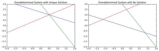
2. Row Interpretation of Over Determined System

Let us consider two small over determined systems and check how we can get an unique solution.

$\begin{bmatrix}1 & 2 \\2 & 1 \\ 2 &-3\end{bmatrix}*\left(\begin{array}{c}x\\ y\end{array}\right)=\begin{bmatrix}5/2 \\2\\-2 \end{bmatrix}$

$\\$

$\begin{bmatrix}1 & 2 \\2 & 1 \\ 2 &-3\end{bmatrix}*\left(\begin{array}{c}x\\ y\end{array}\right)=\begin{bmatrix} 0 \\2\\-4 \end{bmatrix}$

If we look at the row-wise graph of the systems – we can conclude that over determined systems generally do not have a solution, it is rare that we will have a solution to that system. Therefore, we need to look for an approximate solution, process of approximate solution would clear if we explore column wise interpretation of the system.

3. Column Interpretation of Over Determined System

The columns wise system is shown below.

lin_reg_3

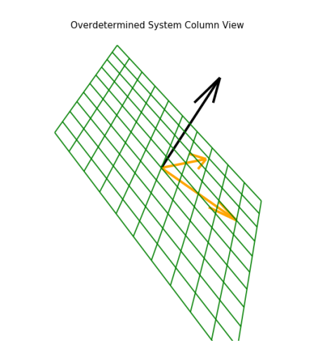
We have plotted the an over-determined system with no solution in the above diagram, clearly vector b of the Ax=b system is not in the columns space of A.Therefore, we cannot have solution,to have solution, b must on the columns space of A. A way out could be approximate b in the columns space as per the diagram above, which we explain in the next figure.

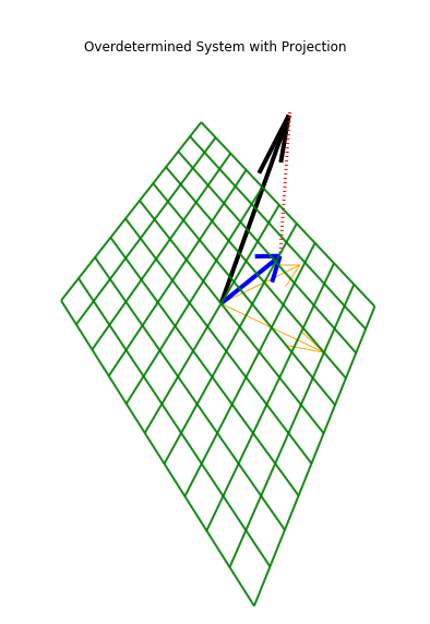
As discussed earlier we can approximate b in the columns space of A, as per the diagram above, which means we make an orthogonal projection of b on the plane which contains both the columns of A. We can construct a new vector (as marked by blue line call it B ) in the diagram. Intuitively the new system that is sitting on the plane containing columns of X could be thought as an approximate solution to the original system. This approximation method of solving the system is known as least square method of solving an over determined system. This idea is key to solving linear regression problem.

In the next section we would extend the idea generated above to establish the following:

How to obtain an approximate solution of the over-determined system, which is the solution for linear regression problem.
Why it is called Least Square
What extra insight we get about regression solution from the column space or observation space visualization.

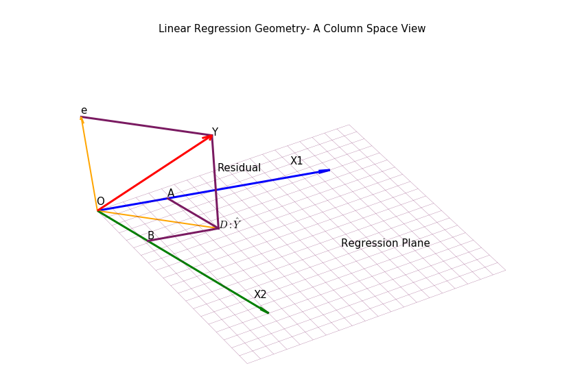
4. Linear Regression Solution Geometry

A typical linear regression problem is like solving an over-determined systems of equations. To have good geometric exposition, we have changed the original problem as multiple regression written in mean deviation form. First record of the changed system is shown below:

$y_0 -\overline{y} = b_1(x_{01}-\overline{x_1})+b_2(x_{02}-\overline{x_2})$

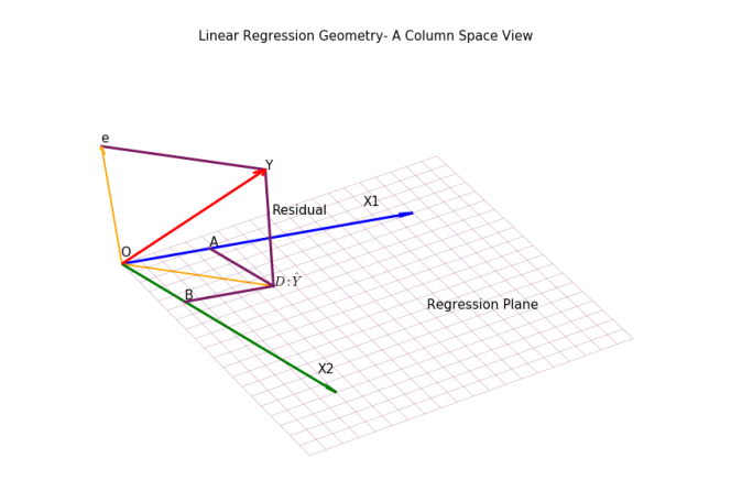
This change is not significant,this has been done make sure our diagram is in conformity with equations written above. With this formulation we depict the regression problem by the following diagram. The diagram below would be valid in generic sense even if we do not write the system in mean deviation form.

We have reproduced the regression problem in observation space or columns space,a detail process of drawing this diagram is described . The most important point is Y vector has been decomposed into two orthogonal component vectors,we can write:

$\overrightarrow{Y}= \overrightarrow{e}+\overrightarrow{\widehat{Y}}$

$\overrightarrow{e}= \overrightarrow{Y}-\overrightarrow{\widehat{Xb}}$

It is obvious from the diagram,error or residual is orthogonal to both X1 and X2. Using the matrix-vector product notation we can write:

$X'*(Y-Xb)=0$ or
$X'X*b = X'Y$

If we analyze the above equation – we would see that this is 2X2 system, therefore,we can solve the system and it will have an unique solution. This form of equation is known as Normal Equations – as we residual is normal to regression plane. A more compact form would be:

$b = (X'X)^{-1} X'Y$

One point we need to clarify why the method described above is called Least Square Method .. let us develop the concept why it is called so .

$E= \sum(e_i^2) = (Y-Xb)'(Y-Xb)=Y'Y -2b'X'Y +b'X'Xb$

In the expression above,we have developed a relation between total sum of squares of the residuals,basically we are collecting residual from each observation,then square and sum…now if we want to tweak it as minimization problem,we ask the question which value of b would minimize the sum of square of residuals??. A little bit calculus would prove that first order condition of the minimization would be lead to the normal equations of above – which means we will get to the same solution, therefore the above method could be called Least Square Solution for over determined systems of equations, which also the solution approch for linear regression problem.

5. Linear Regression Insights from Geometry

In addition to the solution approch, many others statistical relations, concepts and lemmas becomes obvious from the picture above, which otherwise requires tedious symbol manipulations.

Total Sum of Squares = Regression Sum of Squares + Residual Sum of Square. Apply Pythagoras theorem on triangle OYD.
$R^2$ measures the Goodness of Fit varies between 0 and 1. A little manipulation of the Sum of Squares relation will get us there.
Cov( $\hat{Y}$ ,e) = 0, We know dot product between the vectors are zero, which means co-variance is zero.
Residual and independent variables are un-correlated. We can extend the orthogonality relation from the picture.
Effect on multiplying X1 by factor k. From the diagram, regression co-eff is the ratio between OA : OX1, if we extend the X1, this ratio will change. So effect will depend on the value of k.

..and many others if we extend this concept further to apply vector space, span and dimension etc. on the diagram above, which would be the topic of another blog.

Another important point that uniqueness of the solution and few other insights are dependent on the fact matrix X is healthy i.e. columns are independent. Independence of columns would ensure X’X is invertible. A lot scenarios might occur where columns of X are not independent,and/or matrix X lacks good properties which would be the matter of discussion under least square computations.

10 members like this