
The following problem appeared as an assignment in the coursera course Algorithm-I by Prof.Robert Sedgewick from the Princeton University few years back (and also in the course cos226 offered at Princeton). The problem definition and the description is taken from the course website and lectures. The original assignment was to be done in java, where in this article both the java and a corresponding python implementation will also be described.
- Use a 2d-tree to support
- efficient range search (find all of the points contained in a query rectangle)
- nearest-neighbor search (find a closest point to a query point).
2d-trees have numerous applications, ranging from classifying astronomical objects to computer animation to speeding up neural networks to mining data to image retrieval. The figure below describes the problem:

2d-tree implementation: A 2d-tree is a generalization of a BST to two-dimensional keys. The idea is to build a BST with points in the nodes, using the x– and y-coordinates of the points as keys in strictly alternating sequence, starting with the x-coordinates, as shown in the next figure.
- Search and insert. The algorithms for search and insert are similar to those for BSTs, but at the root we use the x-coordinate (if the point to be inserted has a smaller x-coordinate than the point at the root, go left; otherwise go right); then at the next level, we use the y-coordinate (if the point to be inserted has a smaller y-coordinate than the point in the node, go left; otherwise go right); then at the next level the x-coordinate, and so forth.
- The prime advantage of a 2d-tree over a BST is that it supports efficient implementation of range search and nearest-neighbor search. Each node corresponds to an axis-aligned rectangle, which encloses all of the points in its subtree. The root corresponds to the entire plane [(−∞, −∞), (+∞, +∞ )]; the left and right children of the root correspond to the two rectangles split by the x-coordinate of the point at the root; and so forth.
- Range search: To find all points contained in a given query rectangle, start at the root and recursively search for points in both subtrees using the following pruning rule: if the query rectangle does not intersect the rectangle corresponding to a node, there is no need to explore that node (or its subtrees). That is, search a subtree only if it might contain a point contained in the query rectangle.
- Nearest-neighbor search: To find a closest point to a given query point, start at the root and recursively search in both subtrees using the following pruning rule: if the closest point discovered so far is closer than the distance between the query point and the rectangle corresponding to a node, there is no need to explore that node (or its subtrees). That is, search a node only if it might contain a point that is closer than the best one found so far. The effectiveness of the pruning rule depends on quickly finding a nearby point. To do this, organize the recursive method so that when there are two possible subtrees to go down, you choose first the subtree that is on the same side of the splitting line as the query point; the closest point found while exploring the first subtree may enable pruning of the second subtree.
- k-nearest neighbors search: This method returns the k points that are closest to the query point (in any order); return all n points in the data structure if n ≤ k. It must do this in an efficient manner, i.e. using the technique from kd-tree nearest neighbor search, not from brute force.
- BoidSimulator: Once the k-nearest neighbors search we can simulate boids: how a flock of birds flies together and a hawk predates. Behold their flocking majesty.The following figures show the theory that are going to be used, taken from the lecture slides of the same course.
Results
The following figures and animations show how the 2-d-tree is grown with recursive space-partioning for a few sample datasets.
- Circle 10 dataset


 />
/>


 />
/> >
>
- Circle 100 dataset


The following figure shows the result of the range search algorithm on the same dataset after the 2d-tree is grown. The yellow points are the points found by the algorithm inside the query rectangle shown.

The next animations show the nearest neighbor search algorithm for a given query point(the fixed white point with black border: the point (0.3, 0.9)) and how the the branches are traversed and the points (nodes) are visited in the 2-d-tree until the nearest neighbor is found.
The next animation shows how the kd-tree is traversed for nearest-neighbor search for a different query point (0.04, 0.7).

The next figures show the result of k-nearest-neighbor search, by extending the previous algorithm with different values of k (15, 10, 5 respectively).
Runtime of the algorithms with a few datasets in Python
As can be seen from the next figure, the time complexity of 2-d tree building (insertion), nearest neighbor search and k-nearest neighbor query depend not only on the size of the datasets but also on the geometry of the datasets.

Applications
Flocking Boids simulator
The flocking boids simulator is implemented with 2-d-trees and the following 2 animations (java and python respectively) shows how the flock of birds fly together, the black / white ones are the boids and the red one is the predator hawk.
Implementing a kNN Classifier with kd tree from scratch
Training phase
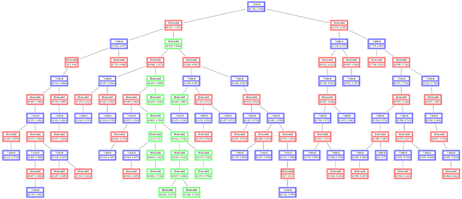
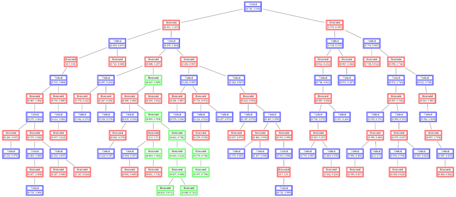
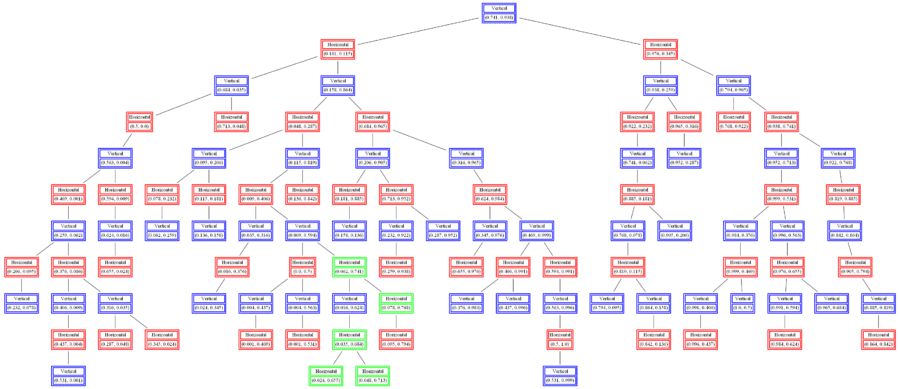
Build a 2d-tree from a labeled 2D training dataset (points marked with red or blue represent 2 different class labels).
Testing phase
- For a query point (new test point with unknown class label) run k-nearest neighbor search on the 2d-tree with the query point (for a fixed value of k, e.g., 3).
- Take a majority vote on the class labels of the k-nearest neighbors (with known class labels) obtained by querying the 2d-tree. Label the query point with the class label that majority of its neighbors have.
- Repeat for different values of k.
The following figures show how the kd tree built can be used to classify (randomly generated) 2D datasets and the decision boundaries are learnt with k=3, 5 and 10respectively.


