price = -55089.98 + 87.34 engineSize + 60.93 horse power + 770.42 width

The model predicts or estimates price (target) as a function of engine size, horsepower, and width (predictors). The model has all the predictors as numeric values.

What if there are qualitative variables? How can the qualitative variables be used in enhancing the models? How are the qualitative variables interpreted?

These are the few questions this blog post will answer.

Fernando gets two such qualitative variables:

• fuelType: The type of fuel used. The value can be gas or diesel.
• driveWheels: The type of drive wheel. It has three values 4 wheels (4WD), rear wheel (RWD) and front wheel (FWD).

The data set looks like this.

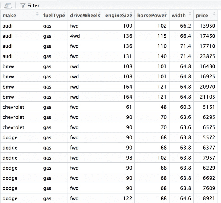
Fernando wants to find out the impact these qualitative variables have on the price of the car.

Concept:

Qualitative variables are variables that are not numerical. It fits the data into categories. They are also called as categorical variables or factors.

Factors have levels. Levels are nothing but unique values of the specific qualitative variables.

• Fuel type has two unique values. Gas or diesel. This implies that there are two factors in fuel type.
• Drive wheels have three unique values. Four when drive, rear wheel drive and front wheel drive. It means that drive wheel has three factors.

Let us look at an example. The sample data has 5 cars, and each car has a diesel or gas fuel type.

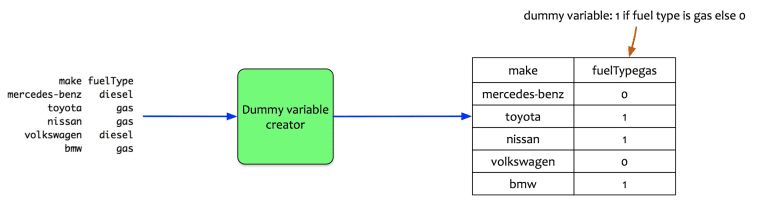
The fuel type is a qualitative variable. It has two levels (diesel or gas). The statistical package creates one dummy variable. It creates a dummy variable named fuelTypegas. This variable takes 0 or 1 value. If the fuel type is gas, then the dummy variable is 1 else it is 0.

Mathematically, it can be written as:

• xi = 1 if fuel type is gas
• xi = 0 is fuel type is diesel

The number of dummy variables created by the regression model is one less than the number factor values in the qualitative variables.

Let us examine how does it manifest in a regression model. A simple regression model with only price and fuel type as input provides the following coefficients:

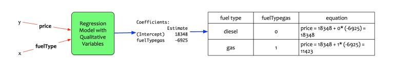
It says the following:

• If the dummy variable is 0 i.e. the fuel type of the car is diesel then price = 18348 + 0 x (-6925) = $18348
• If the dummy variable is 1 i.e. the fuel type of the car is gas then price = 18348 + 1 x (-6925) = $11423

The way qualitative variables with two-factor levels is treated is clear. How about variables with more than two levels? Let us examine another example to understand it.

The drive wheel is a qualitative variable with three factors. In this case, the regression model creates two dummy variables. Let us look at an example. The sample data has 4 cars.

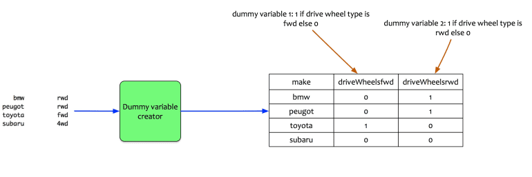
Two dummy variables are created:

• driveWheelsfwd : 1 if drive wheel type is FWD else 0
• driveWheelsrwd: 1 if drive wheel type is RWD else 0

Mathematically, it can be written as:

• xi1 = 1 if the drive wheel is forward; 0 if the drive wheel is not forward.
• xi2 = 1 if the drive wheel is rear; 0 if the drive wheel is not the rear.

Note that there is no dummy variable for 4WD.

How do they manifest in the regression model? The way the regression model treats them is as follows:

• First, it creates a baseline for the price estimation. The baseline is the average price for the qualitative variable for which no dummy variable is created. It is the intercept value. Baseline equation is for 4WD. It is the average price of a 4WD car.
• For FWD: The average price for front wheel drive (fwd) is estimated as baseline + 1 x coefficient of FWD. i.e. price = 7603 + 1 x 1405 + 0 x 10704 = $9008. It means that on an average, an FWD car costs $1405 more than a 4WD.
• For RWD: The price for rear wheel drive (red) is estimated as baseline + 1 x coefficient of RWD. i.e. price = 7603 + 0 x 1405 + 1 x 10704 = $18307. It means that on an average, a rwd car costs $10704 more than a 4WD.

All the qualitative variables with more than two-factor values are treated similarly.

Model Building:

Now that the mechanics of the treatment of qualitative variables. Let us see how does Fernando apply it to his model. His original model was the following:

price = -55089.98 + 87.34 engineSize + 60.93 horse power + 770.42 width

He adds two more qualitative variables into the mix. Fuel type and wheel drive. The general form of the model is written as:

price = β0 + β1.engineSize + β2.horsePower + β3.width + β4.fuelTypegas +β5.driveWheelsfwd + β6.driveWheelsrwd.

Fernando trains the model in his statistical package and gets the following coefficients.

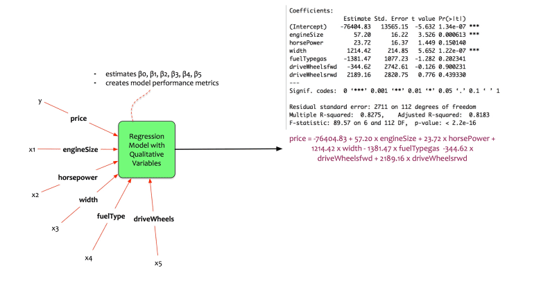
The equation of the model is:

price = -76404.83 + 57.20 * engineSize + 23.72 * horsePower + 1214.42 * width – 1381.47 * fuelTypegas -344.62 * driveWheelsfwd + 2189.16 * driveWheelsrwd

Here there is a mix of quantitative and qualitative variables. The variables are independent of each other. Let us now interpret the coefficients:

• β0: Note that there are no dummy variables created for diesel cars and 4WD cars. β0represents the average price of diesel and 4WD cars. It is a negative value. This implies that if there were 4WD which is diesel, the average price would be a negative value. This is not possible. The model may be violating linear regression assumptions.
• β1: This interpretation is same as the one for multivariate regression. It is interpreted as the average increase in car price if the engine size is increased by 1 unit. An increase of the engine size by 1 unit results in an average increase of car price by $57.
• β2: This interpretation is same as the one for multivariate regression. It is interpreted as the average increase in car price if the horsepower is increased by 1 unit. An increase of the horse power by 1 unit results in an average increase of car price by $23.72.
• β3: This interpretation is same as the one for multivariate regression. It is interpreted as the average increase in car price if the width is increased by 1 unit. An increase of the width by 1 unit results in an average increase of car price by $1214.42.
• β4: This coefficient is the resultant of a dummy variable (fuel type gas). It interpreted as the average difference in price between a diesel fueled car, and gas fueled car. It means that on an average, a car with a fuel type gas will cost $1381.47 lesser than a diesel car.
• β5: This coefficient is the resultant of a dummy variable (drive wheel fwd). It interpreted as the average difference in price between a 4WD and an fwd car. It means that on an average, a car FWD car will cost $344.62 lesser than a 4WD car.
• β6: This coefficient is the resultant of a dummy variable (drive wheel RWD). It interpreted as the average difference in price between a 4WD and an RWD car. It means that on an average, a car RWD car will cost $2189.16 more than a 4WD car.
• Adjusted r-squared is 0.8183. This implies that the model explains 81.83% of the variation in training data.
• Note that not all the coefficients are significant. In fact, in this case, the qualitative variables have no significance on the model performance.

Conclusion:

This model is not better than the original model created. However, it has done its job. We understand the way qualitative variables are interpreted in a regression model. It is evident that the original model with horsepower, engine size and width is better. However, he wonders: horsepower, engine size, and width are treated independently.

What if there are relations between horsepower, engine size and width? Can these relationships be modeled?

The next blog post of this series will address these questions. It will explain the concept of interactions.