
There are many good and sophisticated feature selection algorithms available in R. Feature selection refers to the machine learning case where we have a set of predictor variables for a given dependent variable, but we don’t know a-priori which predictors are most important and if a model can be improved by eliminating some predictors from a model. In linear regression, many students are taught to fit a data set to find the best model using so-called “least squares”. In most exercises in school, all of the data are used in the fit and properties of the model are generated using ANOVA or directly from a regression software. In R, the base function lm() can perform multiple linear regression:
linear_model <- lm(dep_var ~ predictors, data = data)
summary(linear_model)
If we generate some data and a dependent model as here:
data <- as.data.frame(matrix(0, nrow = 100, ncol = 5))
colnames(data) <- c(“time”, “var1”, “var2”, “var3”, “metric”)
data$time <- seq(1, 100, 1)
data$var1 <- sqrt(data$time) * 3 + 11
data$var2 <- 15 * sin(2 * pi * (1/11) * data$time)
data$var3 <- runif(100, -10, 100)
data$metric <- 13 +
0.32 * data$time +
runif(100, 0, 0.05) * 10 * data$var1 +
runif(100, 0, 0.25) * data$var2 +
0.001 * data$var3
then the summary() command produces an output as follows:
Call:
lm(formula = metric ~ ., data = data)
Residuals:
Min 1Q Median 3Q Max
-8.9091 -3.6757 -0.4311 3.4920 10.4595
Coefficients:
Estimate Std. Error t value Pr(>|t|)
(Intercept) 5.815137 6.886533 0.844 0.400555
time 0.229572 0.085726 2.678 0.008728 **
var1 0.592517 0.354949 1.669 0.098350 .
var2 0.168135 0.044888 3.746 0.000309 ***
var3 0.005759 0.014996 0.384 0.701793
—
Signif. codes:
0 ‘***’ 0.001 ‘**’ 0.01 ‘*’ 0.05 ‘.’ 0.1 ‘ ’ 1
Residual standard error: 4.724 on 95 degrees of freedom
Multiple R-squared: 0.8449, Adjusted R-squared: 0.8384
F-statistic: 129.4 on 4 and 95 DF, p-value: < 2.2e-16
One of the great features of R for data analysis is that most results of functions like lm() contain all the details we can see in the summary above, which makes them accessible programmatically. In the case above, the typical approach would be to drop var3, and perhaps var1, and re-fit the data, as those predictors don’t appear to be very significant. However, with just a bit of code, we can do this programmatically and evaluate the results:
threshold <- 0.05
signif_form <-
as.formula(paste(“metric ~ “,
paste(names(which((summary(linear_model)$coefficients[
2:(nrow(summary(linear_model)$coefficients)), 4] < threshold) == TRUE)),
collapse = “+”)))
linear_model <- lm(signif_form, data = data)
summary(linear_model)
Call:
lm(formula = signif_form, data = data)
Residuals:
Min 1Q Median 3Q Max
-9.0971 -3.8859 -0.3897 3.4210 10.1607
Coefficients:
Estimate Std. Error t value Pr(>|t|)
(Intercept) 5.99592 6.83985 0.877 0.382884
time 0.22955 0.08534 2.690 0.008435 **
var1 0.59496 0.35331 1.684 0.095438 .
var2 0.16796 0.04469 3.759 0.000293 ***
—
Signif. codes:
0 ‘***’ 0.001 ‘**’ 0.01 ‘*’ 0.05 ‘.’ 0.1 ‘ ’ 1
Residual standard error: 4.703 on 96 degrees of freedom
Multiple R-squared: 0.8447, Adjusted R-squared: 0.8398
F-statistic: 174 on 3 and 96 DF, p-value: < 2.2e-16
Voila! We now have a model containing only the predictors with significance at the 0.05 level or higher. Note that in the actual data contained within the variable linear_model, the significance values are the exact values vs. the thresholds shown in the summary; therefore we use 0.099 to take all coefficients that would be shown as 0.05 but not 0.01. If we used strict 0.05 as the threshold, a significance of 0.051 would be rejected.
Astute readers will note that the R-squared for the final model is slightly worse than the first, although the adjusted R-squared is slightly better. Back in school, we would have probably focused on the R-squared as the condition of quality, and used the first model. However, in a machine learning context, we are often interested in predicting future, unseen data. That puts additional requirements on the model, and we’ll use another data set to illustrate.
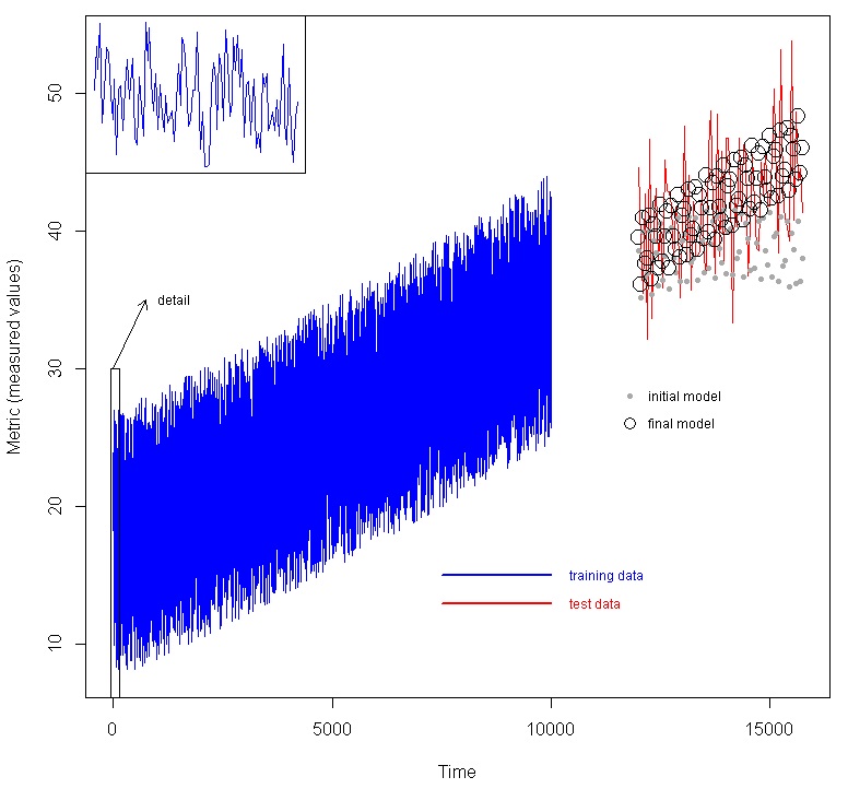
We used a larger, multivariate time-series data set which was divided into training data and test data, where the test data are not presented to the model at all, but we wish to predict them. An example would be where we have collected data on an industrial system, and we wish to build a model to predict future behavior given measured variables. In the figure below, we show a data set with seven factors (time plus 6 other variables) as predictors, and the metric. The blue line are the training data. To illustrate the time varying nature an inset is provided of the first 100 data points. Using the method above, an initial model was created, then feature selection was done, and a final model was created. The red line are the test data, which were generated using the same functions as the test data, but later time. The initial model generated the predictions shown as the grey dots, while the final model generated the predictions shown by the black circles.
These simple examples show some of the power and utility of base R to handle modeling and feature selection. The data and code for the final example are available on github.
%20in%20R)