
This article was written by Steeve Huang.
Reinforcement Learning (RL) refers to a kind of Machine Learning method in which the agent receives a delayed reward in the next time step to evaluate its previous action. It was mostly used in games (e.g. Atari, Mario), with performance on par with or even exceeding humans. Recently, as the algorithm evolves with the combination of Neural Networks, it is capable of solving more complex tasks, such as the pendulum problem.
Although there are a great number of RL algorithms, there does not seem to be a comprehensive comparison between each of them. It gave me a hard time when deciding which algorithms to be applied to a specific task. This article aims to solve this problem by briefly discussing the RL setup, and providing an introduction for some of the well-known algorithms.
Reinforcement Learning 101
Typically, a RL setup is composed of two components, an agent and an environment.
Then environment refers to the object that the agent is acting on (e.g. the game itself in the Atari game), while the agent represents the RL algorithm. The environment starts by sending a state to the agent, which then based on its knowledge to take an action in response to that state. After that, the environment send a pair of next state and reward back to the agent. The agent will update its knowledge with the reward returned by the environment to evaluate its last action. The loop keeps going on until the environment sends a terminal state, which ends to episode.
Most of the RL algorithms follow this pattern. In the following paragraphs, I will briefly talk about some terms used in RL to facilitate our discussion in the next section.
Definition
- Action (A): All the possible moves that the agent can take
- State (S): Current situation returned by the environment.
- Reward (R): An immediate return send back from the environment to evaluate the last action.
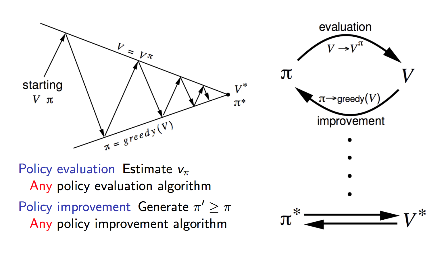
- Policy (π): The strategy that the agent employs to determine next action based on the current state.
- Value (V): The expected long-term return with discount, as opposed to the short-term reward R. Vπ(s) is defined as the expected long-term return of the current state sunder policy π.
- Q-value or action-value (Q): Q-value is similar to Value, except that it takes an extra parameter, the current action a. Qπ(s, a) refers to the long-term return of the current state s, taking action a under policy π.
Model-free v.s. Model-based
The model stands for the simulation of the dynamics of the environment. That is, the model learns the transition probability T(s1|(s0, a)) from the pair of current state s0 and action a to the next state s1. If the transition probability is successfully learned, the agent will know how likely to enter a specific state given current state and action. However, model-based algorithms become impractical as the state space and action space grows (S * S * A, for a tabular setup).
On the other hand, model-free algorithms rely on trial-and-error to update its knowledge. As a result, it does not require space to store all the combination of states and actions. All the algorithms discussed in the next section fall into this category.
On-policy v.s. Off-policy
An on-policy agent learns the value based on its current action a derived from the current policy, whereas its off-policy counter part learns it based on the action a* obtained from another policy. In Q-learning, such policy is the greedy policy. (We will talk more on that in Q-learning and SARSA)
To read the whole article, with illustrations, click here. This article describes the following techniques:
- Q-Learning
- State-Action-Reward-State-Action (SARSA)
- Deep Q Network (DQN)
- Deep Deterministic Policy Gradient (DDPG)