

In the lingo of artificial intelligence, subjecting the machine learning models to real-world environments wherein they can act on the real-world data and generate the prognostications for the real-world problems is called “operationalizing” the machine learning models.

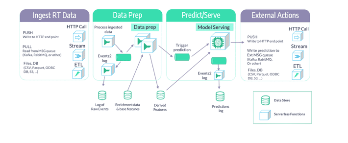
(Flowchart of machine learning process and pipeline building & monitoring)
Exploratory data analysis helps you analyze your machine learning models and data sets involved to bring out the main characteristics by often using graphics and other data visualization methods. The main purpose of EDA is to look at data before making any assumptions. It can help one figure out the obvious errors, as well as better understand the patterns within data to detect outliers and to detect anonymous events, even to find interesting relationships among variables.
EDA assists in building better ML models, as it is used to gauze beyond what lies with conventional modeling or hypothesis testing tasks and provides marketers with a better understanding of data set variables and relationships between them. It can also help determine whether the statistical techniques that one is using for data analysis are appropriate.
Feature engineering, on the other hand, facilitates the machine learning process by increasing the predictive power of machine learning algorithms by creating features from raw data. The method involves leveraging data mining techniques to extract features from raw data along with the use of domain knowledge and is useful to improve the performance of the machine learning algorithms. Often considered applied machine learning, feature engineering offers two important advantages: a) reduced complexity and b) algorithms being fed on raw data to build the models.
Operationalizing machine learning is amongst the culminating stages before deploying and running an ML model in a production environment.
After training a machine learning model the DevOps team needs to operationalize it and this turns out to be a significant challenge for many enterprises. Operationalizing your machine learning model is all about subjecting your model to real-world environments to provide predictive insights for real-world problems. One of the key points to remember while operationalizing your machine learning models is that you must focus on data quality and data management to be relevant for AI operationalization.
The “operationalization” of your ML model might be thought of as a transition phase in between the development and training stages which take place in the training environment using cleaned data, and the deployment and management stages. This becomes especially relevant when the model runs in one of many different business application environments using messy and real-world data.
Operationalization in short is also referred to as “o16n,” because the word is too big.
(Steps to creating, training, and operationalizing your ML Pipeline)
How to Operationalize Your Machine Learning Models
Operationalizing your machine learning model can be a complex process that encompasses the steps below:
- Selection of a use case for ML model
- Deciding on the acceptable probability ranges for determining predictions
- Calculation of the computation power that the model will require when implemented in the real-world scenarios
- Discovering the best ways to resolve issues such as explainability; usually operationalized models deliver high accuracy at the expense of explainability
- Serving the ML model by establishing the full data pipelines
- Hyperparameter tuning and configurations for iterative improvement
- Building a model scoring engine
- Deploying the model correctly in the chosen business application context
- Data cleansing followed by the model evaluation to suit the real-world scenarios and developing a new training data set
- Monitoring the model performance
- Analyzing the results of the models and figuring out errors if any and retraining the model when needed
The operationalization of the machine learning models is usually assisted by the DevOps or MLOps teams whereas the data science and data engineering teams are responsible for developing & training the model and for the continuous monitoring and improvement of the CI/CD pipelines.
Pre-requisites for Operationalizing Your Machine Learning Models
Machine learning models can bring a lot of value to enterprises across every vertical; however, to actualize those values businesses must optimize their machine learning model.
One of the core challenges that machine learning projects encounter is that the data science teams can end up in a silo of pure ML modeling.
While it’s easy to produce beautiful models a lot of effort is required to understand and decipher real-world business value through the model. For businesses to benefit from ML models, they must operationalize their models and with regard to the context in which they will be deployed. Models once operationalized are deployed in a business application, and then are subjected to data analysis and predictive modeling.
Core Challenges of Operationalizing the ML Models
- Data Science and Operations Teams Might Work in Silos
The teams operationalizing your machine learning models may use different tools, concepts, and tech stacks as compared to the data scientists who trained those models which may be one of the prime challenges. Transitioning from training to operationalizing environments can be a struggle.
- ML Models Might Be Oblivious About the Real World Issues
Data scientists focus on what they do. They may not always take into consideration other issues that impact the way the ML models are deployed in the real world such as legal, compliance, IT Ops, or data architecture restrictions that can instigate some essential changes to the way the model operates. Under such circumstances, the business analysts’ team or Ops teams need to accommodate and address such challenges without affecting the efficacy of the model.
How Amazon SageMaker Data Wrangler Helps in Operationalizing Your Data Flow into Your ML Pipeline
A survey called, ‘The State of Data Science 2020,’ revealed that data management, exploratory data analysis (EDA), feature selection & feature engineering account for more than 66% time of a data scientist.
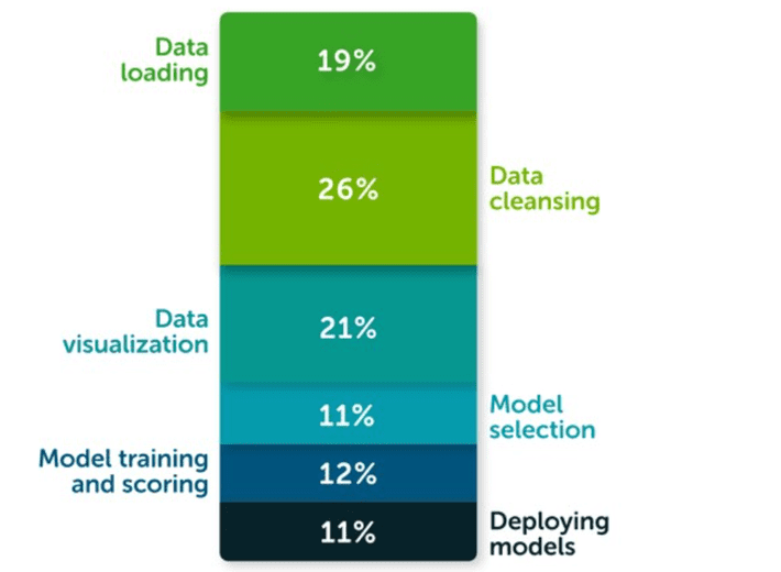
(Diagram showing the percentage of time allocated by a data scientist to different tasks)
The same survey highlights that the top 3 biggest roadblocks to deploying a model in production are managing dependencies and environments, security, and bridging the skill gaps.
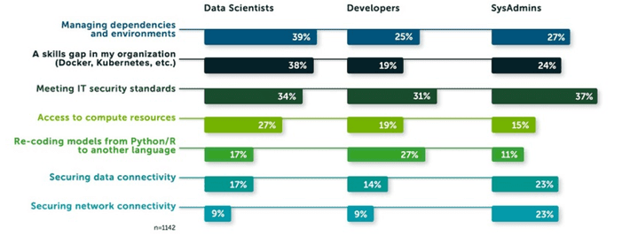
(Diagram showing the three biggest roadblocks to deploying an ML model)
The survey establishes that these struggles enable as many as 48% of the respondents to comprehend and illustrate the impact of data science on business outcomes.
The top advantage of using Amazon SageMaker Data Wrangler is that it is the fastest and easiest way to prepare data for machine learning (ML). With SageMaker Data Wrangler marketers can:
- Use a visual interface to access data, perform EDA and feature engineering, and can seamlessly operationalize their data flow by exploiting it into an Amazon SageMaker pipeline, Amazon SageMaker Data Wrangler job, Python file, or SageMaker feature group
- SageMaker Data Wrangler also provides marketers with over 300 built-in transforms, custom transforms using a Python, PySpark, or SparkSQL runtime, built-in data analysis such as common charts (like scatterplot or histogram), custom charts using Altair library, and useful model analysis capabilities such as feature importance, target leakage, and model explainability
- With the help of SageMaker, one can also create a data flow file that can be versioned and shared across all your teams for reproducibility
Generating Sample Dataset
Now let’s have a look at how we can use a retail demo store example and generate a sample dataset. We use three files: users.csv, items.csv, and interactions.csv.
Firstly, we prepare the data in order to predict the customer segment based on past interactions. Suppose the target field is called persona, which can later be transformed and renamed as USER_SEGMENT.
The following code is a preview of
id,username,email,first_name,last_name,addresses,age,gender,persona
1,user1,[email protected],Nathan,Smith,”[{“”first_name””: “”Nathan””, “”last_name””: “”Smith””, “”address1″”: “”049 Isaac Stravenue Apt. 770″”, “”address2″”: “”””, “”country””: “”US””, “”city””: “”Johnsonmouth””, “”state””: “”NY””, “”zipcode””: “”12758″”, “”default””: true}]”,28,M,electronics_beauty_outdoors
2,user2,[email protected],Kevin,Martinez,”[{“”first_name””: “”Kevin””, “”last_name””: “”Martinez””, “”address1″”: “”074 Jennifer Flats Suite 538″”, “”address2″”: “”””, “”country””: “”US””, “”city””: “”East Christineview””, “”state””: “”MI””, “”zipcode””: “”49758″”, “”default””: true}]”,19,M,electronics_beauty_outdoors
The following code is preview of the items dataset:
ITEM_ID,ITEM_URL,ITEM_SK,ITEM_NAME,ITEM_CATEGORY,ITEM_STYLE,ITEM_DESCRIPTION,ITEM_PRICE,ITEM_IMAGE,ITEM_FEATURED,ITEM_GENDER_AFFINITY
36,http://dbq4nocqaarhp.cloudfront.net/#/product/36,,Exercise Headphones,electronics,headphones,These stylishly red ear buds wrap securely around your ears making them perfect when exercising or on the go.,19.99,5.jpg,true, 49,http://dbq4nocqaarhp.cloudfront.net/#/product/49,,Light Brown Leather Lace-Up Boot,footwear,boot,Sturdy enough for the outdoors yet stylish to wear out on the town.,89.95,11.jpg,,
The following code is a preview of the interactions dataset:
ITEM_ID,USER_ID,EVENT_TYPE,TIMESTAMP
2,2539,ProductViewed,1589580300
29,5575,ProductViewed,1589580305
4,1964,ProductViewed,1589580309
46,5291,ProductViewed,1589580309
Now let’s move towards the process of preparing a training dataset and highlight some of the transformers and data analysis capabilities using Amazon SageMaker Data Wrangler. One can download the .flow files if one intends to download, upload and retrace the full example in his SageMaker Studio environment.
One needs to follow the steps below:
- Connect to Amazon S3 (Amazon Simple Storage Service) and import the data
- Transform the data by including typecasting, dropping unneeded columns, imputing the missing values, label coding, one hot encoding, and custom transformations to extract elements from a JSON formatted column
- Conduct data analysis by creating table summaries and charts. The quick model option can be used to get a sense of the features adding predictive power as one progresses with data preparation. One can also employ the in-build target leakage capability and can generate a report on any features that are at risk of leaking
- One can create a data flow in which one can combine and join three tables to perform further aggregations and data analysis
- Iterations can be performed by additional feature engineering or data analysis on the newly added data
- Thereafter, the workflow can be exported to a SageMaker Data Wrangler job.
Prerequisites
One needs to ensure that there are not any quota limits on the m5.4xlarge instance type part of their Studio application before creating a new data flow. One can refer to the documentation: Getting Started with Data Wrangler for more information on the prerequisites.
Importing the Data
One can import the three CSV files from Amazon S3. SageMaker Data Wrangler supports CSV and Parquet files. One can also sample the data if it is too large to fit in your studio application.
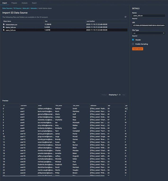
(A preview of users’ dataset)
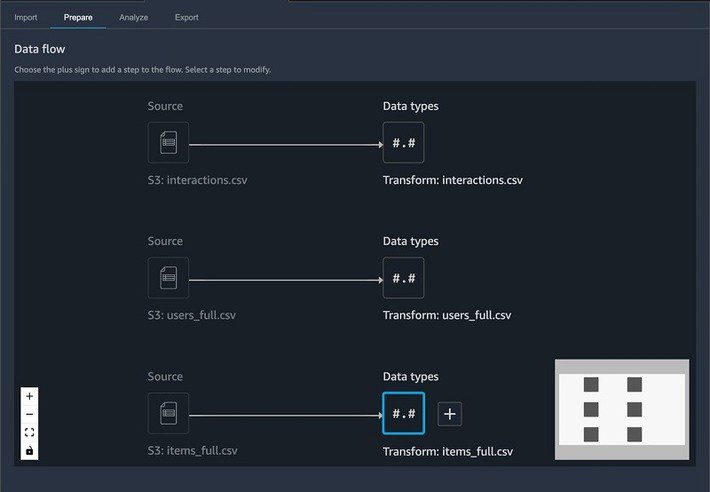
(After importing CSV files, our dataset looks like the picture above in SageMaker Data Wrangler)
One can now add the transformers and get started with data analysis.
Transforming the Data
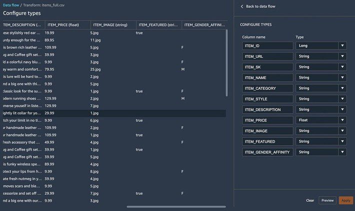
For each of the tables, we check the data types and ensure that it has been correctly inferred.
Items Table
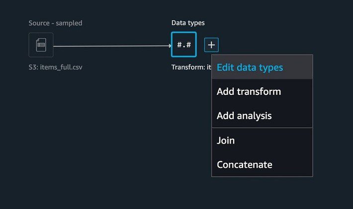
To perform transforms on the items table, one needs to complete the following steps:
- Choose + on the SageMaker Data Wrangler UI, for the items table.
- Choose Edit data types.
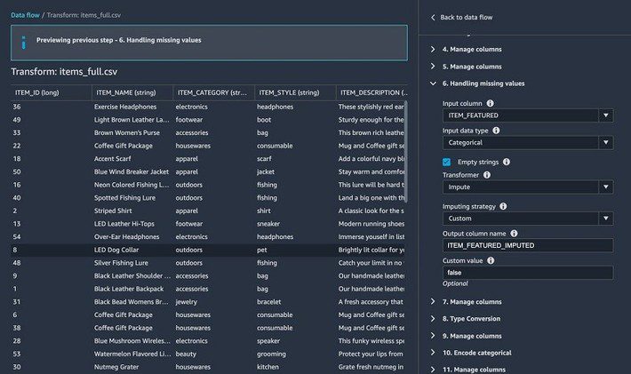
Most of the columns were inferred properly, except for one. The ITEM_FEATURED column is missing values and should really be cast as a Boolean.
For the items table, we perform the following transformations:
- Fill missing values with false for the ITEM_FEATURED column
- Drop unnecessary columns such as URL, SK, IMAGE, NAME, STYLE, ITEM_FEATURED, and DESCRIPTION
- Rename ITEM_FEATURED_IMPUTED to ITEM_FEATURED
- The ITEM_FEATURED column should be cast as Boolean
- Encode the ITEM_GENDER_AFFINITY column
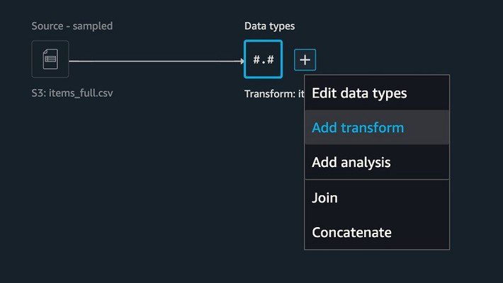
3. To add a new transform, choose + and choose ‘Add transform‘.
 4. Fill in missing values using the built-in Handling missing values transform.
5. To drop columns, under Manage columns, For the Input column, choose ITEM_URL.
- For Required column operator, choose Drop column.
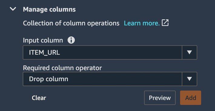
- Repeat this step for URL, SK, IMAGE, NAME, STYLE, ITEM_FEATURED and DESCRIPTION
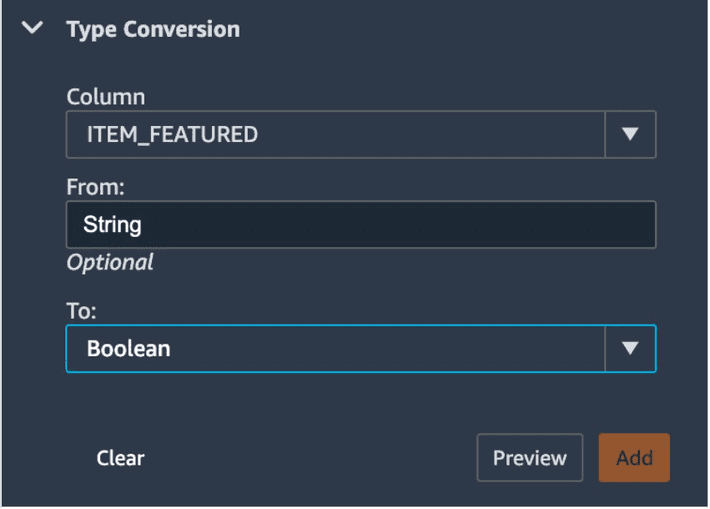
6. Under Type Conversion for Column, choose ITEM_FEATURED.
7. For To, choose Boolean.
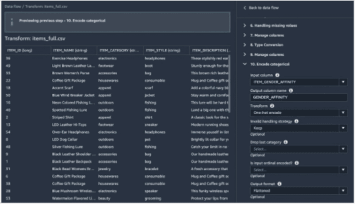
8. Under Encore categorical, add a one hot encoding transform to the ITEM_GENDER_AFFINITY
 9. Rename our column from
ITEM_FEATURED_IMPUTED to ITEM_FEATURED
10. Run a table summary.
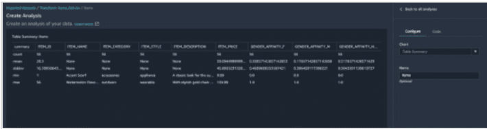
The table summary data analysis doesn’t provide you with the information on all columns.
- Run the info() function as a custom transform.
- Choose Preview to verify that the ITEM_FEATURED column comes as a Boolean data type.
DataFrame.info() prints information about the DataFrame including the data types, non-null values, and memory usage.
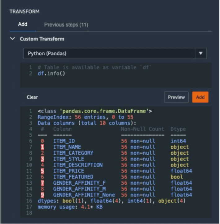
- Check that the ITEM_FEATURED column has been properly cast and is devoid of any null values.
We now move on to the users table and prepare the dataset for training.
Users Table
For the users table, we must perform the following steps:
- The non-essential columns such as username, email, first_name, and last_name must be dropped.
- The elements must be extracted from a JSON column such as zip code, state, and city.
The addresses column containing a JSON string looks like the following code:
[{ “first_name”: “Nathan”,
“last_name”: “Smith”,
“address1”: “049 Isaac Stravenue Apt. 770”,
“address2”: “”,
“country”: “US”,
“city”: “Johnsonmouth”,
“state”: “NY”,
“zipcode”: “12758”,
“default”: true
}]
To extract relevant location elements for our model, we apply several transforms and save them in their respective columns.
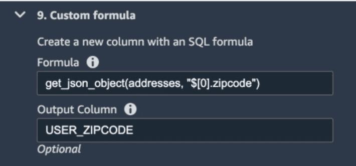
(An example of extracting the user zip code)
We apply the same transform to extract city and state, respectively.
- In the following transform, we split and rearrange the different personas (such as electronics_beauty_outdoors) and save it as USER_SEGMENT.
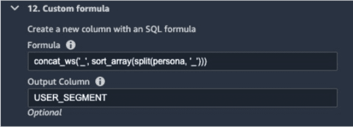
(Splitting, rearrangement, and saving of different personas)
- One can also perform one hot encoding on the USER_GENDER
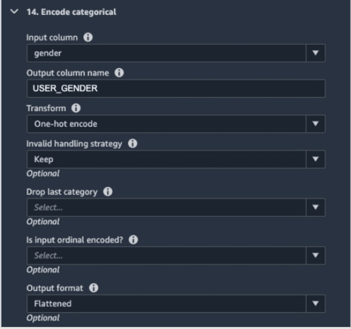
(Performing hot encoding on the USER_GENDER column)
Interactions table
Finally, in the interactions table, we complete the following steps:
- Perform a custom transform to extract the event date and time from a timestamp.
Custom transforms are quite powerful because they allow the end-users to in set a snippet of code and run the transform using different runtime engines such as PySpark, Python, or SparkSQL. The only thing that the users need to do is to start their transform with df which stands for DataFrame.
The following code is an example of using a custom PySpark transform to extract the date and time from the timestamp:
from pyspark.sql.functions import from_unixtime, to_date, date_format
df = df.withColumn(‘DATE_TIME’, from_unixtime(‘TIMESTAMP’))
df = df.withColumn( ‘EVENT_DATE’, to_date(‘DATE_TIME’)).withColumn( ‘EVENT_TIME’, date_format(‘DATE_TIME’, ‘HH:mm:ss’))
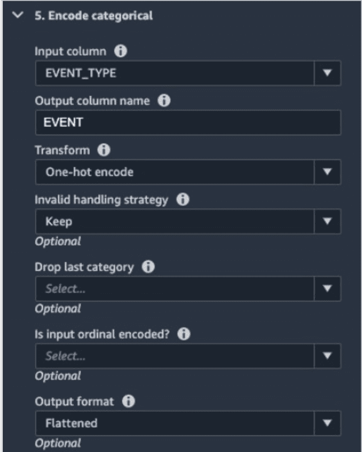
- Perform a one hot encoding on the EVENT_TYPE
- Lastly, one needs to drop the columns that one doesn’t need.
Performing Data Analysis
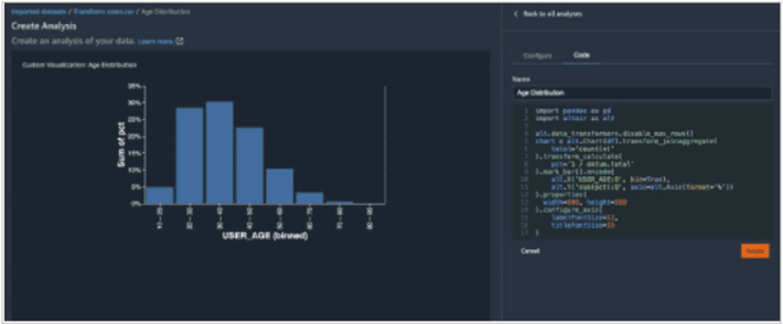
Besides having the common in-built data analysis competencies such as scatterplots and histograms, SageMaker Data Wrangler allows the ends users to build custom visualizations using the Altair library.
In the following histogram chart, we binned the user by age ranges on the x-axis and the total percentage of users on the y axis.
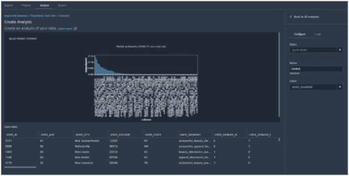
End-users can also use the quick model functionality to show feature importance. The F1 score indicating the model’s predictive accuracy can be seen in the visualization below:
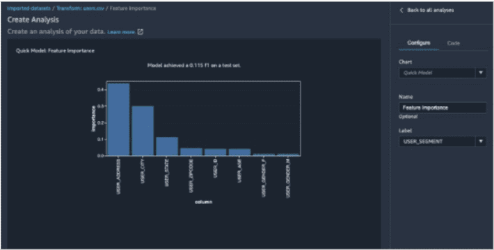
This allows the users to iterate by adding new datasets and performing additional features engineering to incrementally improve model accuracy.
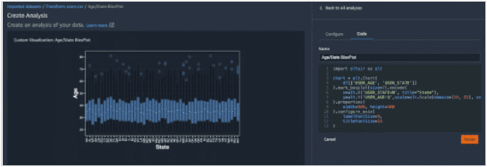
The following visualization is a box plot by age and state. This helps marketers understand the interquartile range and possible outliers.
Building a Data Flow
SageMaker Data Wrangler builds a data flow and keeps the dependencies of all the transforms, data analysis, and table joins. This allows marketers to keep a lineage of their exploratory data analysis and also allows them to replicate the past experiences consistently.
Let’s deep delve into how to join interactions and item tables.
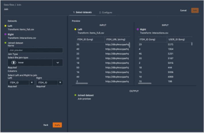
- We join our tables using the ITEM_ID key
- We use a custom transform to aggregate our dataset by USER_ID and generate other features by pivoting the ITEM_CATEGORY and EVENT_TYPE:
import pyspark.sql.functions as F
df = df.groupBy([“USER_ID”]).pivot(“ITEM_CATEGORY”)
.agg(F.sum(“EVENT_TYPE_PRODUCTVIEWED”).alias(“EVENT_TYPE_PRODUCTVIEWED”),
F.sum(“EVENT_TYPE_PRODUCTADDED”).alias(“EVENT_TYPE_PRODUCTADDED”),
F.sum(“EVENT_TYPE_CARTVIEWED”).alias(“EVENT_TYPE_CARTVIEWED”),
F.sum(“EVENT_TYPE_CHECKOUTSTARTED”).alias(“EVENT_TYPE_CHECKOUTSTARTED”),
F.sum(“EVENT_TYPE_ORDERCOMPLETED”).alias(“EVENT_TYPE_ORDERCOMPLETED”),
F.sum(F.col(“ITEM_PRICE”) * F.col(“EVENT_TYPE_ORDERCOMPLETED”)).alias(“TOTAL_REVENUE”),
F.avg(F.col(“ITEM_FEATURED”).cast(“integer”)).alias(“FEATURED_ITEM_FRAC”),
F.avg(“GENDER_AFFINITY_F”).alias(“FEM_AFFINITY_FRAC”),
- F.avg(“GENDER_AFFINITY_M”).alias(“MASC_AFFINITY_FRAC”)).fillna(0)
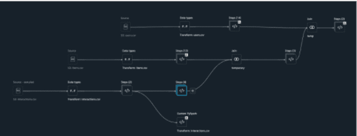
(What DAG looks like after joining all the tables together)
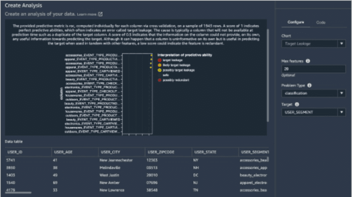
- After combining all three tables, the data analysis needs to be run for target leakage.
Target leakage or data leakage is amongst the most common and difficult problems when building a model. Target leakages mean that marketers use features as part of training their model that isn’t available upon inference time. For instance, if one tries to predict a car crash and one of the features is airbag_deployed, one can’t know whether the airbag has been deployed until the crash happens.
The following screenshot shows that we don’t have a strong target leakage candidate after running the data analysis.
- Finally, we run a quick model on the joined dataset.
The picture below shows that our F1 score is 0.89 after joining additional data and performing further feature transformations.
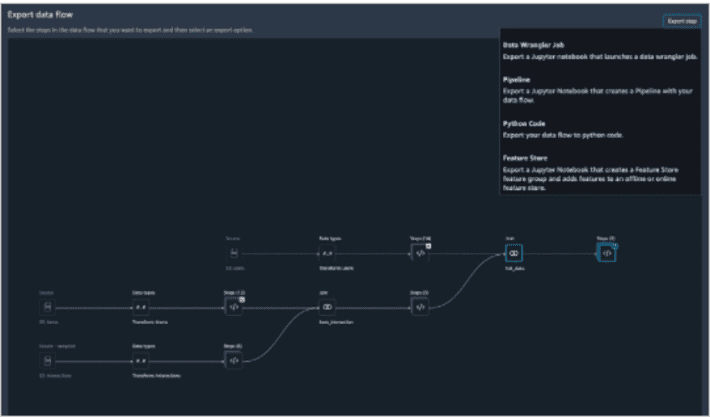
Exporting Your Data Flow
With SageMaker Data Wrangler, one gets equipped to export the data flow into Jupyter notebook with code pre-populated for the following options:
- SageMaker Data Wrangler job
- SageMaker Pipelines and
- SageMaker Feature Store
SageMaker Data Wrangler can also output a Python file.
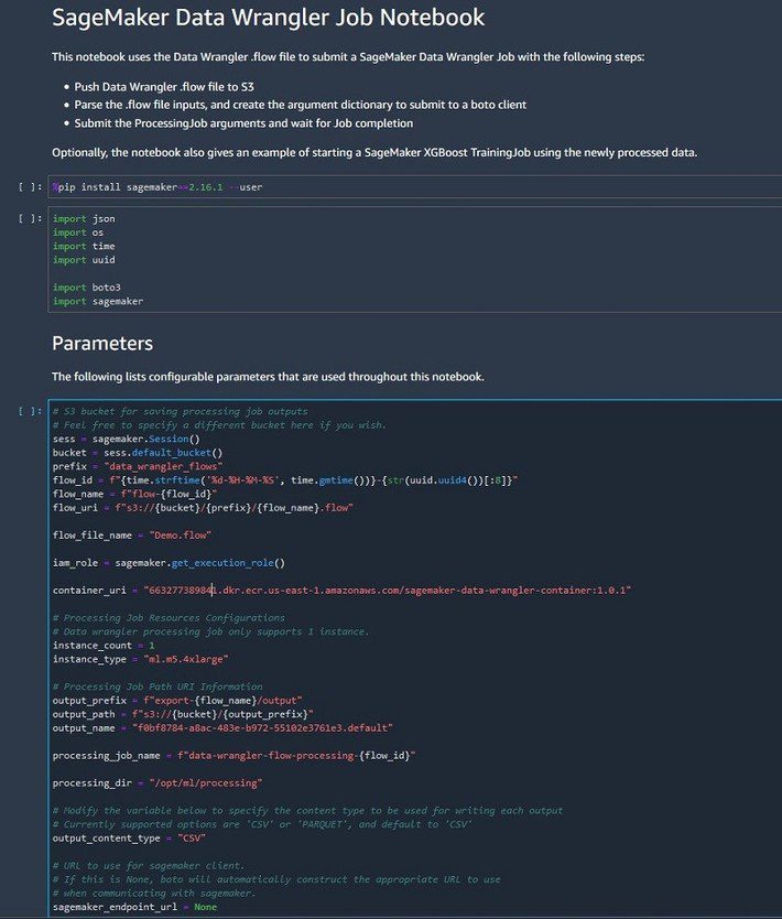
The SageMaker Data Wrangler job pre-populates in the Jupyter notebook and is ready to be run.
Benefits of Using AWS SageMaker Data Wrangler for Operationalizing Your Machine Learning Models
- Creation of end-to-end Machine Learning Pipelines – With the help of AWS SageMaker Data Wrangler one can create the machine learning pipelines that gather and process data, train models, and operationalize and deploy models, instead of siloing each step in separate departments.
- Automate Data Pipelines – Automated machine learning pipelines can gather and process relevant data, monitor model performance, find new training datasets, and more and all of these functionalities are easily workable with Amazon SageMaker. Automating the workflows frees up a lot of time for your MLOps teams, data scientists, analysts, and other people closely intertwined and working with the operations department.
- Improve Collaboration – When the entire process takes place on a single platform, it eases communication, coordination, and collaboration between your data science and analysts teams and your ops teams, supporting easier and scalable execution and deployment of the ML models.
- Data-Driven Decision Making – Operationalizing your ML models with the help of AWS SageMaker Data Wrangler ensures that one can enjoy business value from them by utilizing them to drive better decision-making, performing risk assessment, spotting opportunities, and doing much more across every line of the business. The faster the marketers can reach this sweet spot, the more benefits they can enjoy from investing in data science and AI.
Wrap Up
SageMaker Data Wrangler simplifies the data ingestion process and facilitates the data ingestion and preparation process. Few of the tasks include exploratory data analysis, feature selection, feature engineering, and more advanced data analysis such as feature importance, target leakage, and model explainability using the easy and intuitive user interface. SageMaker Data Wrangler makes the transition of converting your data flow into an operational artifact such as SageMaker Data Wrangler job, SageMaker feature store, or SageMaker pipeline very easy with the click of a button.
%20to%20Operationalize%20Your%20ML%20Pipeline)