
Regression is the first technique you’ll learn in most analytics books. It is a very useful and simple form of supervised learning used to predict a quantitative response.
Originally published on Ideatory Blog.
By building a regression model to predict the value of Y, you’re trying to get an equation like this for an output, Y given inputs x1, x2, x3…
Y= b1.x1 + b2.x2 + b3.x3
Sometimes there may be terms of the form b4x1.x2 + b5.x1^2… that add to the accuracy of the regression model. The trick is to apply some intuition as to what terms could help determine Y and then test the intuition.
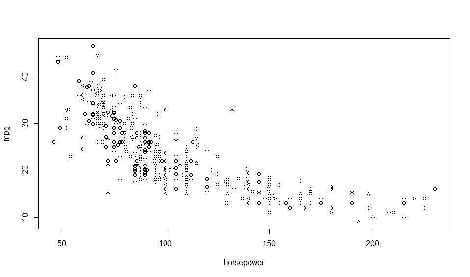
Scatter plots can help you tease out these relationships as we will show in the R section below.
Where is it applicable?
A very common use case is predicting sales from advertising spend on various media. Another common one is predicting house prices based on inputs like sqm/sqft area of the house, the location, number of rooms etc.
Predicting Miles per Gallon from Auto Specifications
I couldn’t find a public dataset for the advertising use-case even though I tried for a while. If you know any such dataset with media-specific advertising spend and sales for the corresponding period with at over 40 or so rows, do share in the comments. I found a dataset on mpg (miles per gallon) on UCI Machine Learning Repository and other car data and regression on that was quite fun.
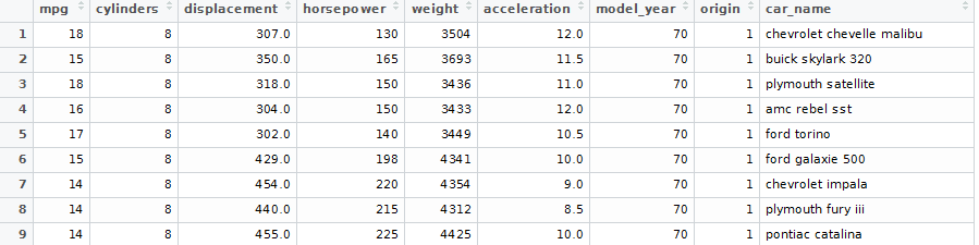
The Dataset
Regression Analysis in RStudio
>auto <- na.omit(read.table("auto-mpg.data"))
>colnames(auto) <- c("mpg","cylinders","displacement","horsepower","weight","acceleration","model_year","origin","car_name")
>auto$horsepower <- as.numeric(levels(auto$horsepower))[auto$horsepower]
>auto <- na.omit(auto)
Use this command to plot pairwise scatter plots in RStudio and inspect the result for relationships between the independent variable mpg and the numerical dependent variables.
>pairs(~mpg + cylinders + displacement + horsepower + weight + acceleration + model_year+origin)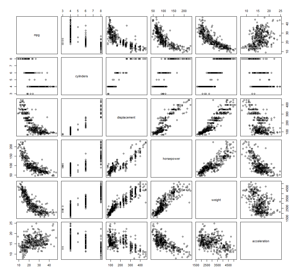
See how quickly a scatter plot helps see the relationships between the variables. Mpg decreases with increase in number of cylinders, displacement, weight, horsepower and increases with acceleration (the variable acceleration represents time taken to acceleration from 0 – 60 mph, so the higher the acceleration value, the worse the actual acceleration).
Your plot would also show relationships among mpg, model-year and origin variables. I excluded them here because the plot image about would become too large to be easily intelligible.
The Regression Modeling Process
Since mpg clearly depends on all the variables, let derive a regression model, which is simple to do in RStudio.
Let’s try a few models:
auto.fit
>auto.fit <- lm(mpg~. -car_name,data=auto)
>summary(auto.fit)
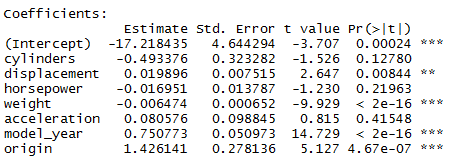
Multiple R-squared: 0.8215, Adjusted R-squared: 0.8182
P-values for coefficients of cylinders, horsepower and acceleration are all greater than 0.05. This means that the relationship between the dependent and these independent variables is not significant at the 95% certainty level. I’ll drop 2 of these variables and try again. High p-values for these independent variables do not mean that they definitely should not be used in the model. It could be that some other variables are correlated with these variables and making these variables less useful for prediction (check Multicollinearity).
auto.fit1
> auto.fit1 <- lm(mpg ~ displacement + horsepower + weight , data=auto)
> summary(auto.fit1)
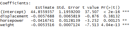
Multiple R-squared: 0.707, Adjusted R-squared: 0.7047
Here we see that both Multiple R-squared and Adjusted R-squared have fallen. When comparing models, use Adjusted R-squared. That’s because R-squared will increase or stay the same (never decrease) when more independent variables are added. The formula for Adjusted R-squared includes an adjustment to reduce R-squared. If the additional variable adds enough predictive information to the model to counter the negative adjustment then Adjusted R-squared will increase. If the amount of predictive information added is not valuable enough, Adjusted R-squared will reduce.
Let’s try more combinations:
auto.fit2
> auto.fit2 <- lm(mpg ~ acceleration + horsepower + weight, data = auto)
> summary(auto.fit2)
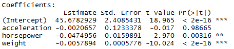
Multiple R-squared: 0.7064, Adjusted R-squared: 0.7041
Trying more combinations as acceleration has very high p-value.
auto.fit3
> auto.fit3 <- lm(mpg ~ model_year + horsepower + weight, data = auto)
> summary(auto.fit3)
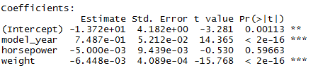
Multiple R-squared: 0.8083, Adjusted R-squared: 0.8068
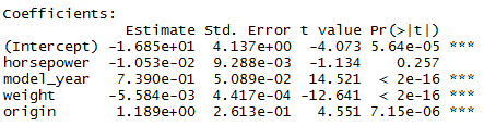
auto.fit4
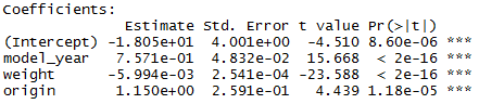
> auto.fit4 <- lm(mpg ~ model_year + horsepower + weight + origin, data = auto)
> summary(auto.fit4)
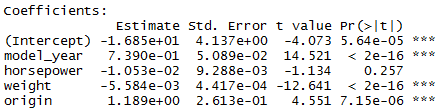
Multiple R-squared: 0.8181, Adjusted R-squared: 0.8162
auto.fit5
> auto.fit5 <- lm(mpg ~ model_year + acceleration + weight + origin, data = auto)
> summary(auto.fit5)
Multiple R-squared: 0.8181, Adjusted R-squared: 0.8162
auto.fit6
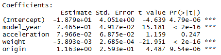
> auto.fit6 <- lm(mpg ~ model_year + weight + origin, data = auto)
> summary(auto.fit6)
Multiple R-squared: 0.8175, Adjusted R-squared: 0.816
Now we’re getting somewhere as all the coefficients have a small p-value.
auto.fit7
> auto.fit7 <- lm(mpg ~ I(displacement^2) + model_year + weight + origin, data = auto)
> summary(auto.fit7)
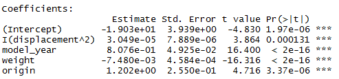
Multiple R-squared: 0.8242, Adjusted R-squared: 0.8224
Let’s try some non-linear combinations with different exponents for horsepower.
auto.fit8
 > auto.fit8 <- lm(mpg ~ I(horsepower^1) + I(horsepower^2) + I(horsepower^3) +
 model_year + weight + origin, data = auto)
> summary(auto.fit8)
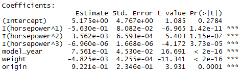
Multiple R-squared: 0.8571, Adjusted R-squared: 0.8548
The Adjusted R-squared is the highest so far. Another thing to note is that even though the p-value for horsepower^3 is very small (relationship is significant), the coefficient is tiny. So we should consider removing it unless horsepower^3 has an intuitive or business meaning to us in the given context.
While creating models we should always bring business understanding into consideration. If the context dictates that that particular variable is important to explaining the outcome, we will retain it in the model even if the coefficient is very small.
If the effect is small and we are not able to explain why the independent variable should affect the dependent variable in a particular way, we may be risking overfitting to our particular sample of data. Such a model may not generalize.
Let’s try just a few more combinations:
auto.fit9
> auto.fit9 <- lm(mpg ~ horsepower + model_year + weight + origin, data = auto)
> summary(auto.fit9)
Multiple R-squared: 0.8181, Adjusted R-squared: 0.8162
Adjusted R-squared reduced. We can do better.
auto.fit10
> auto.fit10 <- lm(mpg ~ model_year + weight + origin + poly(horsepower,2) , data=auto)
> summary(auto.fit10)
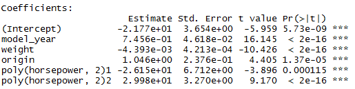
Multiple R-squared: 0.8506, Adjusted R-squared: 0.8487
There we go. This is a good enough model. Adjusted R-squared is the second highest. None of the coefficients seem miniscule. The coefficient for weight is quite small compared to the others but the weight values are in thousands. So, the effect in reality is quite significant. Also, intuition dictates that mpg should be dependent on the weight of the vehicle. So even if the effect were small, we would have kept it.
mpg = – 21.77 + 0.7456e*model_year – 0.004393*weight + 1.046*origin – 26.15*horsepower^1 + 29.98*horsepower^2
Useful Questions to ask of the Dataset
These are based on the excellent analysis in “An Introduction to Statistical Learning” textbook. Let’s use the model obtained to answer the questions.
- Is there a relationship between mpg and other variables?
There seems to be a strong relationship between mpg (represented above as the dependent variable) and the independent variables model_year, weight, origin and horsepower.
- How strong is the relationship?
The relationship is quite strong as 85% of the variance in the dependent variable is explained by these independent variables.
- Which specifications contribute to raising or lowering mpg?
We see that weight and horsepower^1 lower mpg. Model_year and origin raise mpg.
- How accurately can we estimate the effect of each specification on mpg?
We are able to estimate the effect of model_year, weight, origin and horsepower on mpg with high accuracy in auto.fit10 model as the p-values for all the included independent variables are much less than 0.05. The variables not included had values larger than 0.05 or had a very small coefficient compared to the others. We could not estimate or isolate the effect of cylinders, displacement and acceleration accurately.
- How accurately can we predict mpg from the given data?
We’re able to explain 85% of the variation in mpg from the auto.fit10 regression model derived from the given data.
To calculate 95% prediction interval of mpg for a given set of values for the independent variables, use the code below.
 newdata <- data.frame(model_year=70, weight=3691, origin=1, horsepower = 200)
 predict(auto.fit10, newdata, interval = "confidence")
fit lwr upr
1 15.03982 13.83341 16.24623This means that for the given values of model_year, weight, origin and horsepower, the mpg will lie between 13.8 and 16.2 with a 95% probability.
- Is the relationship linear?
The relationship is non-linear between mpg and horsepower.
Results
We were able to explain 85% of the variance in miles per gallon using the regression model below. Intuition agrees with this model as weight and horsepower would definitely affect mpg. A surprising finding was that model_year and origin had significant effects also.
mpg = – 21.77 + 0.7456e*model_year – 0.004393*weight + 1.046*origin – 26.15*horsepower^1 + 29.98*horsepower^2
Appendix:
Info about the dataset from UCI Machine Learning Repository
- Title: Auto-Mpg Data
- Sources:
Origin: This dataset was taken from the StatLib library which is maintained at Carnegie Mellon University. The dataset was used in the 1983 American Statistical Association Exposition.Date: July 7, 1993
- Past Usage:
– See 2b (above)
– Quinlan,R. (1993). Combining Instance-Based and Model-Based Learning. In Proceedings on the Tenth International Conference of Machine Learning, 236-243, University of Massachusetts, Amherst. Morgan
Kaufmann. - Relevant Information:
This dataset is a slightly modified version of the dataset provided in the StatLib library. In line with the use by Ross Quinlan (1993) in predicting the attribute “mpg”, 8 of the original instances were removed
because they had unknown values for the “mpg” attribute. The original
dataset is available in the file “auto-mpg.data-original”.“The data concerns city-cycle fuel consumption in miles per gallon, to be predicted in terms of 3 multivalued discrete and 5 continuous attributes.” (Quinlan, 1993)
- Number of Instances: 398
- Number of Attributes: 9 including the class attribute
- Attribute Information:
- mpg: continuous
- cylinders: multi-valued discrete
- displacement: continuous
- horsepower: continuous
- weight: continuous
- acceleration: continuous
- model year: multi-valued discrete
- origin: multi-valued discrete
- car name: string (unique for each instance)
- Missing Attribute Values: horsepower has 6 missing values